Prediction

Overview

By the end of this practical you will know how to:

Fit regression, decision trees and random forests to training data.
Evaluate model fitting and prediction performance in a test set.
Compare the fitting and prediction performance of two models.
Explore the effects of features on model predictions.

Tasks

A - Setup

Open your TheRBootcamp R project. It should already have the folders 1_Data and 2_Code. Make sure that the data file(s) listed in the Datasets section are in your 1_Data folder.
Open a new R script and save it as a new file called Prediction_practical.R in the 2_Code folder.
Using library() load the set of packages for this practical listed in the packages section above.

# Load packages necessary for this script
library(rpart.plot)
library(tidyverse)
library(tidymodels)
tidymodels_prefer() # to resolve common conflicts

We will again work with the airbnb data. Load the dataset using the code below.

# airbnb data
airbnb <- read_csv(file = "1_Data/airbnb.csv")

You should already be familiar with the dataset, but you can refresh your memory by checking the variable names with names() and the contents using View().

B - Splitting the data into training and test set

In the previous practical, we used the complete airbnb dataset to fit the models. To avoid over-fitting, we will now split the data into a training- and a test-set. Use the initial_split() function to create a split. Pass it the airbnb data as argument and save the output as airbnb_split.

# initialize split
XX <- XX(XX)

airbnb_split <- initial_split(airbnb)

Create a training-set using the training() function. Pass it the airbnb_split object as argument and save the output as airbnb_train.

# training data
XX <- XX(XX)

airbnb_train <- training(airbnb_split)

Create a test-set using the testing() function. Pass it the airbnb_split object as argument and save the output as airbnb_test.

# test data
XX <- XX(XX)

airbnb_test <- testing(airbnb_split)

B - Fitting

Your goal in this set of tasks is again to fit models predicting price, the price of Airbnbs located in Berlin.

Regression

Define a recipe called lm_recipe by calling the recipe() function. Use all available predictors by setting the formula to price ~ . and use the airbnb_train data. Also, add a pipe (%>%) and step_dummy(all_nominal_predictors()) to dummy-code all categorical predictors.

# create recipe
XX <- 
  XX(XX, data = XX) %>% 
  XX(XX())

# create recipe
lm_recipe <- 
  recipe(price ~ ., data = airbnb_train) %>% 
  step_dummy(all_nominal_predictors())

Print the recipe.

lm_recipe

Data Recipe

Inputs:

      role #variables
   outcome          1
 predictor         22

Operations:

Dummy variables from all_nominal_predictors()

Create a regression model by

calling the linear_reg() function.
adding a pipe and setting the enginge to "lm" using set_engine().
specifying the problem mode to "regression" using set_mode().
saving the output as lm_model.

# set up the regression model
XX <- 
  XX() %>% 
  XX(XX) %>% 
  XX(XX)

# set up the regression model
lm_model <- 
  linear_reg() %>% 
  set_engine("lm") %>% 
  set_mode("regression")

Print the model.

lm_model

Linear Regression Model Specification (regression)

Computational engine: lm

Create a workflow called lm_workflow using workflow() and add the lm_recipe and lm_model objects using add_recipe() and add_model().

# lm workflow 
lm_workflow <- 
  XX() %>% 
  XX(XX) %>% 
  XX(XX)

# lm workflow 
lm_workflow <- 
  workflow() %>% 
  add_recipe(lm_recipe) %>% 
  add_model(lm_model)

Print the workflow.

lm_workflow

== Workflow ====================================================================
Preprocessor: Recipe
Model: linear_reg()

-- Preprocessor ----------------------------------------------------------------
1 Recipe Step

* step_dummy()

-- Model -----------------------------------------------------------------------
Linear Regression Model Specification (regression)

Computational engine: lm

Fit the model on the training data by passing the lm_workflow and the airbnb_train data to the fit() function and save the output as price_lm.

# Fit the regression model
XX <-
  XX %>% 
  XX(XX)

# Fit the regression model
price_lm <-
  lm_workflow %>% 
  fit(airbnb_train)

Using the tidy() function on the price_lm object, take a look at the parameter estimates.

# regression model parameters
tidy(price_lm)

# A tibble: 35 x 5
   term                    estimate std.error statistic  p.value
   <chr>                      <dbl>     <dbl>     <dbl>    <dbl>
 1 (Intercept)            -145.       84.6       -1.71  8.80e- 2
 2 accommodates             23.2       2.20      10.5   1.74e-24
 3 bedrooms                 15.3       5.54       2.75  6.00e- 3
 4 bathrooms                20.2       9.00       2.25  2.50e- 2
 5 cleaning_fee             -0.285     0.117     -2.43  1.53e- 2
 6 availability_90_days     -0.0309    0.0941    -0.328 7.43e- 1
 7 host_response_rate       -0.153     0.336     -0.455 6.49e- 1
 8 host_superhostTRUE        9.64      6.29       1.53  1.26e- 1
 9 host_listings_count       0.328     0.674      0.486 6.27e- 1
10 review_scores_accuracy   11.6       7.34       1.58  1.14e- 1
# ... with 25 more rows

Using the predict() function, to extract the model predictions from price_lm and bind them together with the true values from airbnb_train using bind_cols().

# get predicted values from training data
lm_pred <-
  XX %>% 
  XX(XX) %>% 
  XX(airbnb_train %>% select(price))

# get predicted values from training data
lm_pred <-
  price_lm %>% 
  predict(new_data = airbnb_train) %>% 
  bind_cols(airbnb_train %>% select(price))

Using the metrics() function, evaluate the model performance. Pass it the price variable as truth and the .pred variable as estimate.

# evaluate performance
XX(lm_pred, truth = XX, estimate = XX)

# evaluate performance
metrics(lm_pred, truth = price, estimate = .pred)

# A tibble: 3 x 3
  .metric .estimator .estimate
  <chr>   <chr>          <dbl>
1 rmse    standard      77.2  
2 rsq     standard       0.358
3 mae     standard      30.0

Using the following code, plot the fitted against the true value, to judge how well our model performed.

# use the lm_pred object to generate the plot
ggplot(lm_pred, aes(x = .pred, y = price)) + 
  # Create a diagonal line:
  geom_abline(lty = 2) + 
  # Add data points:
  geom_point(alpha = 0.5) + 
  labs(title = "Regression: All Features",
       subtitle = "Line indicates perfect performance",
       x = "Predicted Airbnb Prices in $",
       y = "True Airbnb Prices in $") +
  # Scale and size the x- and y-axis uniformly:
  coord_obs_pred()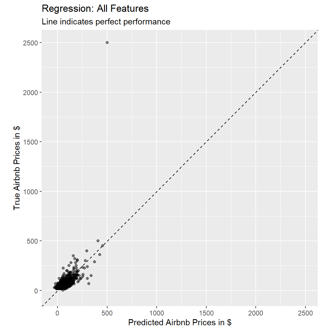

Decision Trees

Decision trees don’t need categorical variables to be dummy coded. Create a new recipe called tree_recipe that uses all available predictors to predict the price of Airbnbs based on the airbnb_train data. In addition, use the pre-proccessing step step_other(all_nominal_predictors(), threshold = 0.005). This will lump together all cases of categorical variables that make up less than 0.5% of the cases into an other category. This will prevent issues when assessing performance using the test set.

tree_recipe <-
  recipe(price ~ ., data = airbnb_train) %>% 
  step_other(all_nominal_predictors(), threshold = 0.005)

Set up a decision tree model. Use the decision_tree() function to specify the model, and set the engine to rpart. Set the mode to "regression". Call the output dt_model.

# set up the decision tree model
XX <- 
  XX() %>% 
  XX(XX) %>% 
  XX(XX)

# set up the decision tree model
dt_model <- 
  decision_tree() %>% 
  set_engine("rpart") %>% 
  set_mode("regression")

Create a new workflow dt_workflow, where you add the newly created tree_recipe and the dt_model.

# decision tree workflow 
dt_workflow <- 
  XX() %>% 
  XX(XX) %>% 
  XX(XX)

# decision tree workflow  
dt_workflow <- 
  workflow() %>% 
  add_recipe(tree_recipe) %>% 
  add_model(dt_model)

Print the workflow.

dt_workflow

== Workflow ====================================================================
Preprocessor: Recipe
Model: decision_tree()

-- Preprocessor ----------------------------------------------------------------
1 Recipe Step

* step_other()

-- Model -----------------------------------------------------------------------
Decision Tree Model Specification (regression)

Computational engine: rpart

Fit the model on the training data by passing the dt_workflow and the airbnb_train data to the fit() function and save the output as price_dt.

# Fit the decision tree
XX <-
  XX %>% 
  XX(XX)

# Fit the decision tree
price_dt <-
  dt_workflow %>% 
  fit(airbnb_train)

The tidy() function won’t work with decision tree fit objects, but we can print the output using the following code:

# print the decision tree output
price_dt %>% 
  extract_fit_parsnip() %>% 
  pluck("fit")

n= 893 

node), split, n, deviance, yval
      * denotes terminal node

1) root 893 8280000  69.7  
  2) accommodates< 11.5 886 1890000  65.4  
    4) accommodates< 4.5 754  708000  54.7  
      8) cleaning_fee< 35.5 585  330000  47.6 *
      9) cleaning_fee>=35.5 169  246000  79.3 *
    5) accommodates>=4.5 132  599000 127.0 *
  3) accommodates>=11.5 7 4280000 617.0 *

Alternatively, we can pass the object you printed in the previous task in the rpart.plot function. This will create a visualization of the decision tree (in this case, the plot does not look very usefull, but depending on the variables used by the model it can be).

price_dt %>% 
  extract_fit_parsnip() %>% 
  pluck("fit") %>% 
  rpart.plot()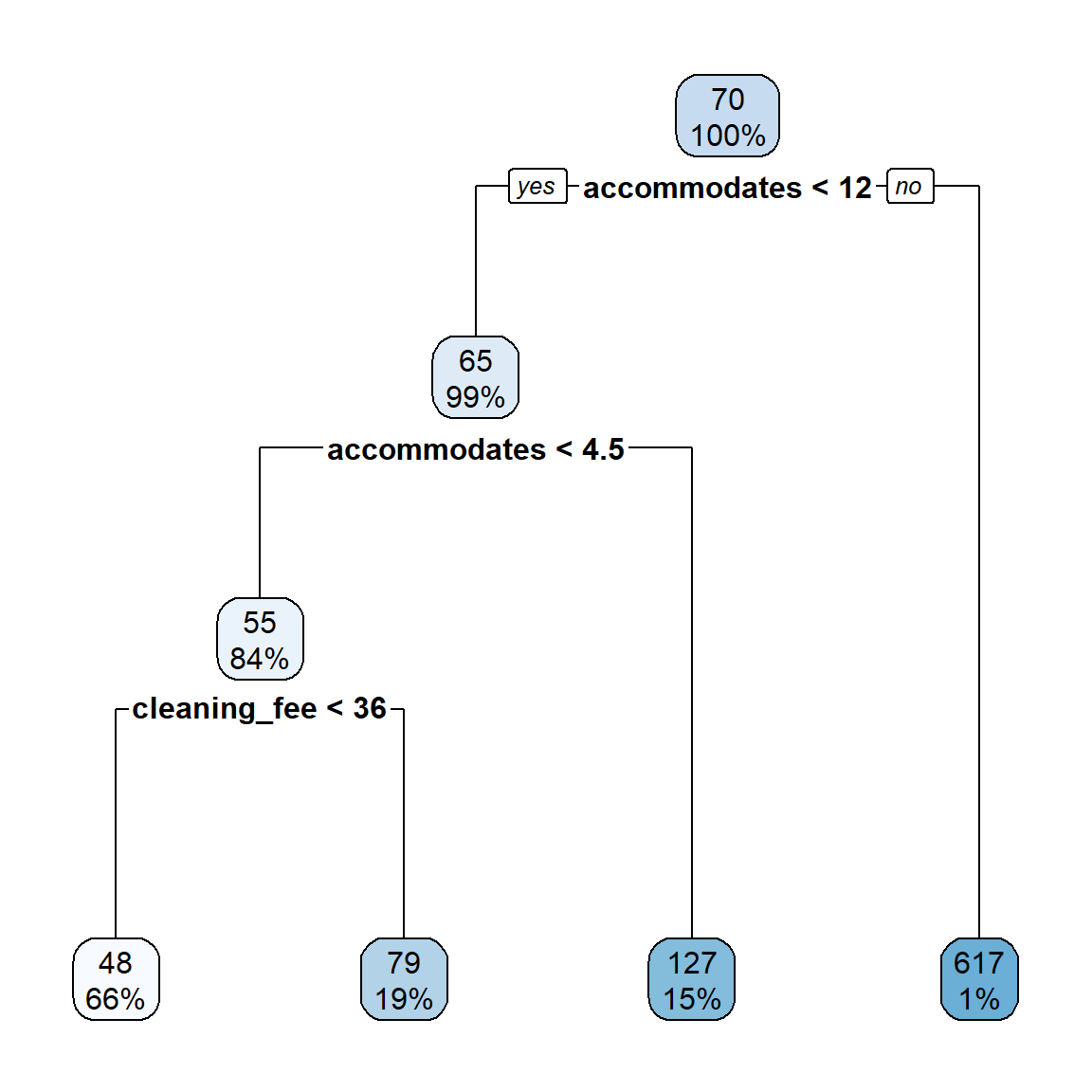

Using the predict() function, to extract the model predictions from price_dt and bind them together with the true values from airbnb_train using bind_cols().

# get predicted values from training data
dt_pred <-
  XX %>% 
  XX(XX) %>% 
  XX(airbnb_train %>% select(price))

# get predicted values from training data
dt_pred <-
  price_dt %>% 
  predict(new_data = airbnb_train) %>% 
  bind_cols(airbnb_train %>% select(price))

Using the metrics() function, evaluate the model performance. Pass it the price variable as truth and the .pred variable as estimate.

# evaluate performance
XX(dt_pred, truth = XX, estimate = XX)

# evaluate performance
metrics(dt_pred, truth = price, estimate = .pred)

# A tibble: 3 x 3
  .metric .estimator .estimate
  <chr>   <chr>          <dbl>
1 rmse    standard      78.2  
2 rsq     standard       0.341
3 mae     standard      28.0

How does the model performance of the decision tree compare to the one of the regression model, based on the training data?
Using the following code, plot the fitted against the true value, to judge how well our model performed.

# use the dt_pred object to generate the plot
ggplot(dt_pred, aes(x = .pred, y = price)) + 
  # Create a diagonal line:
  geom_abline(lty = 2) + 
  # Add data points:
  geom_point(alpha = 0.5) + 
  labs(title = "Decision Tree: All Features",
       subtitle = "Line indicates perfect performance",
       x = "Predicted Airbnb Prices in $",
       y = "True Airbnb Prices in $") +
  # Scale and size the x- and y-axis uniformly:
  coord_obs_pred()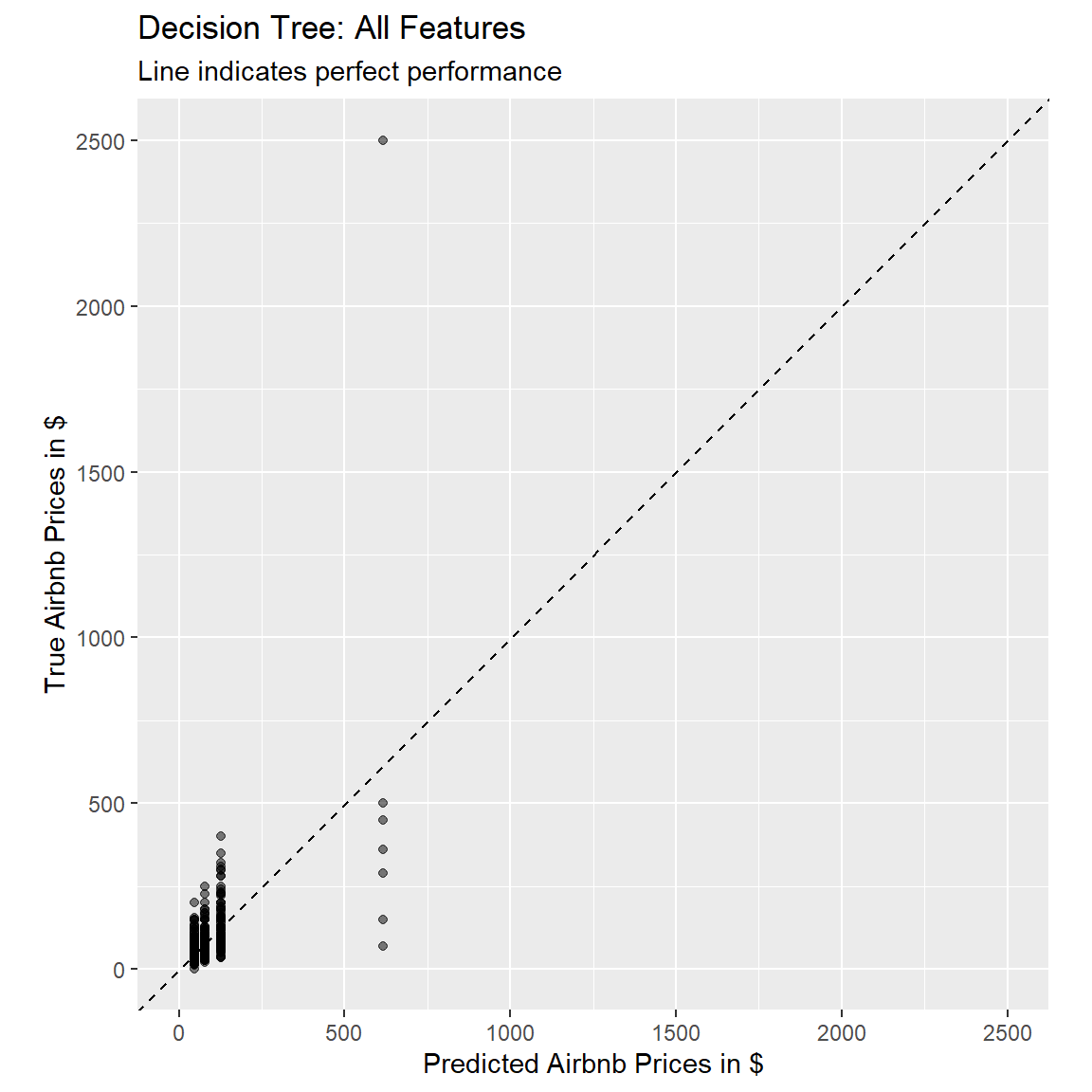

Random Forests

As random forests are made up of many decision trees, we can use the recipe we defined for the decision tree, so we only have to set up a random forest model. Use the rand_forest() function to specify the model, and set the engine to "ranger". Set the mode to "regression". Call the output rf_model.

# set up the random forest model
XX <- 
  XX() %>% 
  XX(XX) %>% 
  XX(XX)

# set up the random forest model
rf_model <- 
  rand_forest() %>% 
  set_engine("ranger") %>% 
  set_mode("regression")

Create a new workflow rf_workflow, where you add the tree_recipe and the newly created rf_model.

# random forest workflow 
rf_workflow <- 
  XX() %>% 
  XX(XX) %>% 
  XX(XX)

# random forest workflow  
rf_workflow <- 
  workflow() %>% 
  add_recipe(tree_recipe) %>% 
  add_model(rf_model)

Print the workflow.

rf_workflow

== Workflow ====================================================================
Preprocessor: Recipe
Model: rand_forest()

-- Preprocessor ----------------------------------------------------------------
1 Recipe Step

* step_other()

-- Model -----------------------------------------------------------------------
Random Forest Model Specification (regression)

Computational engine: ranger

Fit the model on the training data by passing the rf_workflow and the airbnb_train data to the fit() function and save the output as price_rf.

# Fit the random forest
XX <-
  XX %>% 
  XX(XX)

# Fit the random forest
price_rf <-
  rf_workflow %>% 
  fit(airbnb_train)

The tidy() function won’t work with random forest fit objects, but we can print the output using the following code:

# print the random forest output
price_rf %>% 
  extract_fit_parsnip() %>% 
  pluck("fit")

Ranger result

Call:
 ranger::ranger(x = maybe_data_frame(x), y = y, num.threads = 1,      verbose = FALSE, seed = sample.int(10^5, 1)) 

Type:                             Regression 
Number of trees:                  500 
Sample size:                      893 
Number of independent variables:  22 
Mtry:                             4 
Target node size:                 5 
Variable importance mode:         none 
Splitrule:                        variance 
OOB prediction error (MSE):       7487 
R squared (OOB):                  0.193

Using the predict() function, to extract the model predictions from price_rf and bind them together with the true values from airbnb_train using bind_cols().

# get predicted values from training data
rf_pred <-
  XX %>% 
  XX(XX) %>% 
  XX(airbnb_train %>% select(price))

# get predicted values from training data
rf_pred <-
  price_rf %>% 
  predict(new_data = airbnb_train) %>% 
  bind_cols(airbnb_train %>% select(price))

Using the metrics() function, evaluate the model performance. Pass it the price variable as truth and the .pred variable as estimate.

# evaluate performance
XX(rf_pred, truth = XX, estimate = XX)

# evaluate performance
metrics(rf_pred, truth = price, estimate = .pred)

# A tibble: 3 x 3
  .metric .estimator .estimate
  <chr>   <chr>          <dbl>
1 rmse    standard      45.4  
2 rsq     standard       0.819
3 mae     standard      12.9

How does the training performance of the random forest compare to the ones of the other two models?
Using the following code, plot the fitted against the true value, to judge how well our model performed.

# use the rf_pred object to generate the plot
ggplot(rf_pred, aes(x = .pred, y = price)) + 
  # Create a diagonal line:
  geom_abline(lty = 2) + 
  # Add data points:
  geom_point(alpha = 0.5) + 
  labs(title = "Random Forest: All Features",
       subtitle = "Line indicates perfect performance",
       x = "Predicted Airbnb Prices in $",
       y = "True Airbnb Prices in $") +
  # Scale and size the x- and y-axis uniformly:
  coord_obs_pred()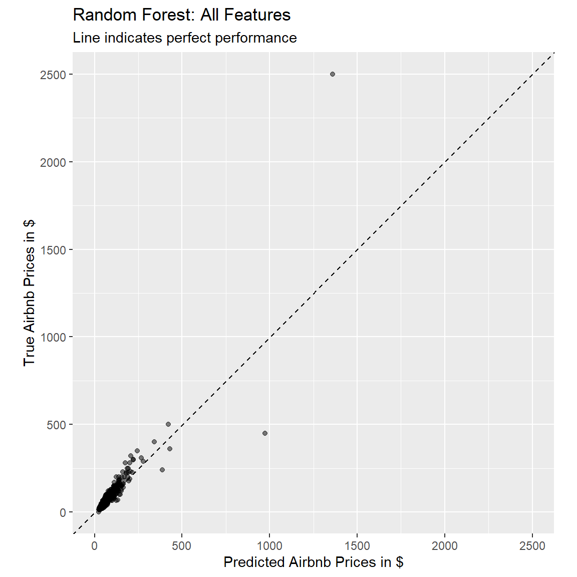

C - Prediction

Before we compared the training performances. Now, let’s compare the out-of-sample performances on the test-set. First the linear regression. Using the predict() function, to extract the model predictions from price_lm, but this time based on airbnb_test and bind them together with the true values from airbnb_test using bind_cols(). Save the output as lm_pred_test

# get predicted values from test data
lm_pred_test <-
  XX %>% 
  XX(XX) %>% 
  XX(airbnb_test %>% select(price))

# get predicted values from test data
lm_pred_test <-
  price_lm %>% 
  predict(new_data = airbnb_test) %>% 
  bind_cols(airbnb_test %>% select(price))

Repeat the step above with the decision tree and random forest fits, to create dt_pred_test and rf_pred_test.

# decision tree
dt_pred_test <-
  price_dt %>% 
  predict(new_data = airbnb_test) %>% 
  bind_cols(airbnb_test %>% select(price))

# random forest
rf_pred_test <-
  price_rf %>% 
  predict(new_data = airbnb_test) %>% 
  bind_cols(airbnb_test %>% select(price))

Using the metrics() function, evaluate the models’ out-of-sample performances. Pass it the price variable as truth and the .pred variable as estimate.

# evaluate performance
XX(XX, truth = XX, estimate = XX)
XX(XX, truth = XX, estimate = XX)
XX(XX, truth = XX, estimate = XX)

# evaluate performance
metrics(lm_pred_test, truth = price, estimate = .pred)

# A tibble: 3 x 3
  .metric .estimator .estimate
  <chr>   <chr>          <dbl>
1 rmse    standard      49.3  
2 rsq     standard       0.524
3 mae     standard      30.2

metrics(dt_pred_test, truth = price, estimate = .pred)

# A tibble: 3 x 3
  .metric .estimator .estimate
  <chr>   <chr>          <dbl>
1 rmse    standard      52.6  
2 rsq     standard       0.483
3 mae     standard      29.0

metrics(rf_pred_test, truth = price, estimate = .pred)

# A tibble: 3 x 3
  .metric .estimator .estimate
  <chr>   <chr>          <dbl>
1 rmse    standard      33.9  
2 rsq     standard       0.799
3 mae     standard      22.3

Which model performs the best based on the test data?

# The random forest predictions are still the most accurate.

Which performance stays the most constant?

# The regression model's performance is very similar in the training and 
# test data. The test performance of the decision tree drops somewhat and
# the test performance of the random forest has the most significant drop
# in comparison to it's training performance.

Which of the three models has the best prediction performance?

# The random forest predictions are still the most accurate.

D - Classification

Let’s again turn to a classification example. We will again focus on the host_superhost variable. Like in the previous practical, we first have to change our criterion to be a factor. We again explicitly specify TRUE as first level.

# Recode host_superhost to be a factor with TRUE as first level
airbnb <-
  airbnb %>% 
  mutate(host_superhost = factor(host_superhost, levels = c(TRUE, FALSE)))

Create a split that balances the proportion of the two levels of host_superhost and that uses 80% of the data for the training.

airbnb_split <- initial_split(XX, prop = XX, strata = XX)

airbnb_split <- initial_split(airbnb, prop = .8, strata = host_superhost)

From the initial split object, creat a training and a test set, and save them as airbnb_train and airbnb_test.

XX <- XX(XX)
XX <- XX(XX)

airbnb_train <- training(airbnb_split)
airbnb_test <- testing(airbnb_split)

F - Fitting

Regression

Specify the recipe for a logistic regression. Specifically…

set the formula to host_superhost ~ ., to use all possible features
use the airbnb_train data
add step_dummy(all_nominal_predictors()) to pre-process nominal features
call the new object logistic_recipe

# create new recipe
XX <- 
  XX(XX, data = XX) %>% 
  XX(XX())

# create new recipe
logistic_recipe <- 
  recipe(host_superhost ~ ., data = airbnb_train) %>% 
  step_dummy(all_nominal_predictors())

Print the new recipe.

logistic_recipe

Data Recipe

Inputs:

      role #variables
   outcome          1
 predictor         22

Operations:

Dummy variables from all_nominal_predictors()

Create a new model called logistic_model, with the model type logistic_reg, the engine "glm", and mode "classification".

# create a logistic regression model 
XX_model <-
  XX() %>% 
  set_XX(XX) %>% 
  set_XX(XX)

# create a logistic regression model 
logistic_model <-
  logistic_reg() %>% 
  set_engine("glm") %>% 
  set_mode("classification")

Create a new workflow called logistic_workflow, where you add the logistic_model and the logistic_recipe together.

# create logistic_workflow 
logistic_workflow <- 
  workflow() %>% 
  add_recipe(logistic_recipe) %>% 
  add_model(logistic_model)

Fit the model on the training data (airbnb_train) using fit(). Save the result as superhost_glm.

# Fit the logistic regression model
superhost_glm <-
  logistic_workflow %>% 
  fit(airbnb_train)

Evaluate the training performance with the metrics() function to do so. First, we again create a dataset containing the predicted and true values. This time, we call the predict() function twice: once to obtain the predicted classes, and once to obtain the probabilities, with which the classes are predicted.

# Get fitted values from the Private_glm object
logistic_pred <- 
  predict(superhost_glm, airbnb_train, type = "prob") %>% 
  bind_cols(predict(superhost_glm, airbnb_train)) %>% 
  bind_cols(airbnb_train %>% select(host_superhost))

Let’s look at different performance metrics. Use the metrics() function and pass it the host_superhost variable as truth, the .pred_class variable as estimate, and .pred_TRUE as last argument.

XX(logistic_pred, truth = XX, estimate = XX, XX)

metrics(logistic_pred, truth = host_superhost, estimate = .pred_class, .pred_TRUE)

# A tibble: 4 x 3
  .metric     .estimator .estimate
  <chr>       <chr>          <dbl>
1 accuracy    binary         0.75 
2 kap         binary         0.483
3 mn_log_loss binary         0.491
4 roc_auc     binary         0.833

Plot the ROC-curve using the roc_curve() function, to create sensitivity and specificity values of different cut-offs, and pass this into the autoplot() function, to plot the curve. Add the host_superhost column as truth, and the .pred_TRUE column as third, unnamed argument, to the roc_curve() function and plot the curve.

XX(logistic_pred, truth = XX, XX) %>% 
  autoplot()

roc_curve(logistic_pred, truth = host_superhost, .pred_TRUE) %>% 
  autoplot()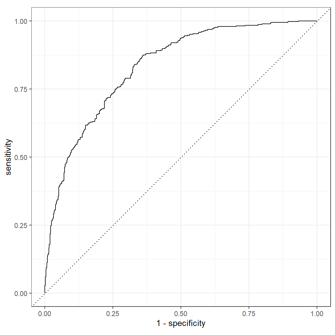

Decision Tree

Create a new recipe called tree_recipe that uses all available predictors to predict host_superhost. In addition, again use the pre-processing step step_other(all_nominal_predictors(), threshold = 0.005).

tree_recipe <-
  recipe(host_superhost ~ ., data = airbnb_train) %>% 
  step_other(all_nominal_predictors(), threshold = 0.005)

Set up a decision tree model. Use the decision_tree() function to specify the model, and set the engine to rpart. Set the mode to "classification". Call the output dt_model.

# set up the decision tree model
dt_model <- 
  decision_tree() %>% 
  set_engine("rpart") %>% 
  set_mode("classification")

Create a new workflow dt_workflow, where you add the newly created tree_recipe and the dt_model.

# decision tree workflow  
dt_workflow <- 
  workflow() %>% 
  add_recipe(tree_recipe) %>% 
  add_model(dt_model)

Print the workflow.

dt_workflow

== Workflow ====================================================================
Preprocessor: Recipe
Model: decision_tree()

-- Preprocessor ----------------------------------------------------------------
1 Recipe Step

* step_other()

-- Model -----------------------------------------------------------------------
Decision Tree Model Specification (classification)

Computational engine: rpart

Fit the model on the training data by passing the dt_workflow and the airbnb_train data to the fit() function and save the output as superhost_dt.

# Fit the decision tree
superhost_dt <-
  dt_workflow %>% 
  fit(airbnb_train)

Evaluate the training performance with the metrics() function to do so. Use the code from the logistic regression above as template. Save the output as dt_pred.

dt_pred <- 
  predict(superhost_dt, airbnb_train, type = "prob") %>% 
  bind_cols(predict(superhost_dt, airbnb_train)) %>% 
  bind_cols(airbnb_train %>% select(host_superhost))

Let’s look at different performance metrics. Use the metrics() function and pass it the host_superhost variable as truth, the .pred_class variable as estimate, and .pred_TRUE as last argument.

metrics(dt_pred, truth = host_superhost, estimate = .pred_class, .pred_TRUE)

# A tibble: 4 x 3
  .metric     .estimator .estimate
  <chr>       <chr>          <dbl>
1 accuracy    binary         0.753
2 kap         binary         0.484
3 mn_log_loss binary         0.552
4 roc_auc     binary         0.754

Plot the ROC-curve using the roc_curve() function, to create sensitivity and specificity values of different cut-offs, and pass this into the autoplot() function, to plot the curve. Add the host_superhost column as truth, and the .pred_TRUE column as third, unnamed argument, to the roc_curve() function and plot the curve.

roc_curve(dt_pred, truth = host_superhost, .pred_TRUE) %>% 
  autoplot()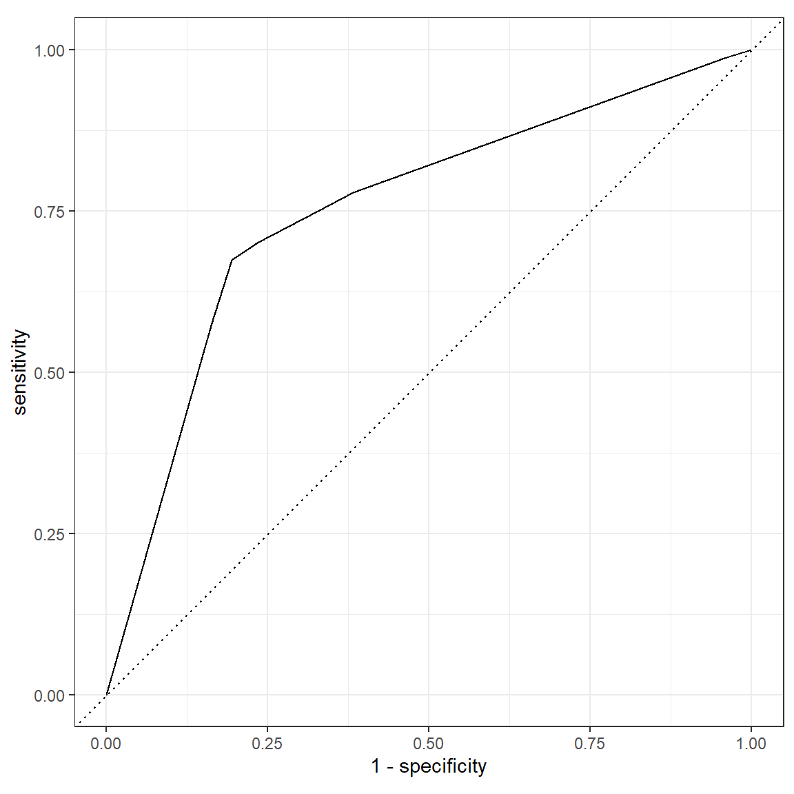

Random Forest

Set up a random forest classification model. Use the rand_forest() function to specify the model, and set the engine to ranger. Set the mode to "classification". Call the output rf_model.

# set up the random forest model
rf_model <- 
  rand_forest() %>% 
  set_engine("ranger") %>% 
  set_mode("classification")

Create a new workflow rf_workflow, where you add the previously created tree_recipe and the new rf_model.

# random forest workflow  
rf_workflow <- 
  workflow() %>% 
  add_recipe(tree_recipe) %>% 
  add_model(rf_model)

Print the workflow.

rf_workflow

== Workflow ====================================================================
Preprocessor: Recipe
Model: rand_forest()

-- Preprocessor ----------------------------------------------------------------
1 Recipe Step

* step_other()

-- Model -----------------------------------------------------------------------
Random Forest Model Specification (classification)

Computational engine: ranger

Fit the model on the training data by passing the rf_workflow and the airbnb_train data to the fit() function and save the output as superhost_rf.

# Fit the random forest
superhost_rf <-
  rf_workflow %>% 
  fit(airbnb_train)

Evaluate the training performance with the metrics() function to do so and save the output as rf_pred.

rf_pred <- 
  predict(superhost_rf, airbnb_train, type = "prob") %>% 
  bind_cols(predict(superhost_rf, airbnb_train)) %>% 
  bind_cols(airbnb_train %>% select(host_superhost))

Let’s look at different performance metrics. Use the metrics() function and pass it the host_superhost variable as truth, the .pred_class variable as estimate, and .pred_TRUE as last argument.

metrics(rf_pred, truth = host_superhost, estimate = .pred_class, .pred_TRUE)

# A tibble: 4 x 3
  .metric     .estimator .estimate
  <chr>       <chr>          <dbl>
1 accuracy    binary         0.961
2 kap         binary         0.919
3 mn_log_loss binary         0.280
4 roc_auc     binary         0.994

Plot the ROC-curve using the roc_curve() function, to create sensitivity and specificity values of different cut-offs, and pass this into the autoplot() function, to plot the curve.

roc_curve(rf_pred, truth = host_superhost, .pred_TRUE) %>% 
  autoplot()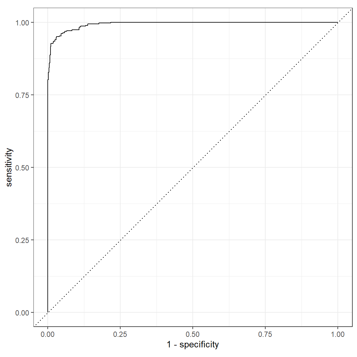

G - Prediction

Before we compared the training performances. Now, let’s compare the out-of-sample performances on the test-set. First the logistic regression. Using the predict() function twice to extract the model predictions from superhost_glm (as done with the training data), but this time based on airbnb_test and bind them together with the true values from airbnb_test using bind_cols(). Save the output as glm_pred_test

# get predicted values from test data
glm_pred_test <-
  superhost_glm %>% 
  predict(airbnb_test, type = "prob") %>% 
  bind_cols(predict(superhost_glm, airbnb_test)) %>% 
  bind_cols(airbnb_test %>% select(host_superhost))

Repeat the step above with the decision tree and random forest fits, to create dt_pred_test and rf_pred_test.

# decision tree
dt_pred_test <-
  superhost_dt %>% 
  predict(airbnb_test, type = "prob") %>% 
  bind_cols(predict(superhost_dt, airbnb_test)) %>% 
  bind_cols(airbnb_test %>% select(host_superhost))

# random forest
rf_pred_test <-
  superhost_rf %>% 
  predict(airbnb_test, type = "prob") %>% 
  bind_cols(predict(superhost_rf, airbnb_test)) %>% 
  bind_cols(airbnb_test %>% select(host_superhost))

Using the metrics() function, evaluate the models’ out-of-sample performances. Pass it the price variable as truth and the .pred variable as estimate.

# evaluate performance
metrics(glm_pred_test, truth = host_superhost, estimate = .pred_class, .pred_TRUE)

# A tibble: 4 x 3
  .metric     .estimator .estimate
  <chr>       <chr>          <dbl>
1 accuracy    binary         0.757
2 kap         binary         0.479
3 mn_log_loss binary         0.476
4 roc_auc     binary         0.845

metrics(dt_pred_test, truth = host_superhost, estimate = .pred_class, .pred_TRUE)

# A tibble: 4 x 3
  .metric     .estimator .estimate
  <chr>       <chr>          <dbl>
1 accuracy    binary         0.749
2 kap         binary         0.459
3 mn_log_loss binary         0.559
4 roc_auc     binary         0.753

metrics(rf_pred_test, truth = host_superhost, estimate = .pred_class, .pred_TRUE)

# A tibble: 4 x 3
  .metric     .estimator .estimate
  <chr>       <chr>          <dbl>
1 accuracy    binary         0.745
2 kap         binary         0.455
3 mn_log_loss binary         0.498
4 roc_auc     binary         0.832

Which model performs the best based on the test data?

# The random forest predictions are still the most accurate.

Plot the ROC-curves of the test performances.

roc_curve(glm_pred_test, truth = host_superhost, .pred_TRUE) %>% 
  autoplot()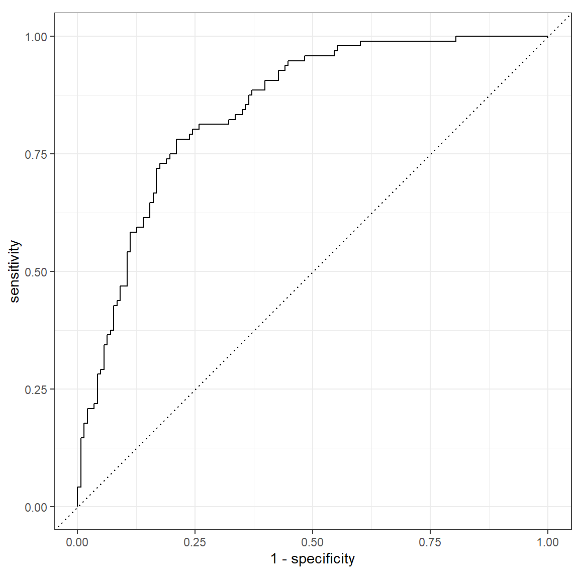

roc_curve(dt_pred_test, truth = host_superhost, .pred_TRUE) %>% 
  autoplot()

roc_curve(rf_pred_test, truth = host_superhost, .pred_TRUE) %>% 
  autoplot()

Examples

# Fitting and evaluating a regression model ------------------------------------

# Step 0: Load packages---------------------------------------------------------
library(tidyverse)    # Load tidyverse for dplyr and tidyr
library(tidymodels)   # For ML mastery 
tidymodels_prefer()   # To resolve common conflicts

# Step 1: Load and Clean, and Explore Training data ----------------------------

# I'll use the mpg dataset from the dplyr package 
# Explore training data
mpg        # Print the dataset
View(mpg)  # Open in a new spreadsheet-like window 
dim(mpg)   # Print dimensions
names(mpg) # Print the names

# Step 2: Split the data--------------------------------------------------------

mpg_split <- initial_split(mpg)
data_train <- training(mpg_split)
data_test <- testing(mpg_split)

# Step 3: Define recipe --------------------------------------------------------

# The recipe defines what to predict with what, and how to pre-process the data
lm_recipe <- 
  recipe(hwy ~ year + cyl + displ + trans,  # Specify formula
         data = data_train) %>%             # Specify the data
  step_dummy(all_nominal_predictors())      # Dummy code all categorical predictors


# Step 4: Define model ---------------------------------------------------------

# The model definition defines what kind of model we want to use and how to
# fit it
lm_model <- 
  linear_reg() %>%        # Specify model type
  set_engine("lm") %>%    # Specify engine (often package name) to use
  set_mode("regression")  # Specify whether it's a regressio or classification
                          #  problem.

# Step 5: Define workflow ------------------------------------------------------

# The workflow combines model and recipe, so that we can fit the model
lm_workflow <- 
  workflow() %>%             # Initialize workflow
  add_model(lm_model) %>%    # Add the model to the workflow
  add_recipe(lm_recipe)      # Add the recipe to the workflow

# Step 6: Fit the model --------------------------------------------------------

hwy_lm <- 
  lm_workflow %>%   # Use the specified workflow
  fit(data_train)   # Fit the model on the specified data

tidy(hwy_lm)        # Look at summary information

# Step 7: Assess fit -----------------------------------------------------------

# Save model predictions and observed values
lm_fitted <- 
  hwy_lm %>%               # Model from which to extract predictions
  predict(data_train) %>%  # Obtain predictions, based on entered data (in this
                           #  case, these predictions are not out-of-sample)
  bind_cols(data_train %>% select(hwy))  # Extract observed/true values

# Obtain performance metrics
metrics(lm_fitted, truth = hwy, estimate = .pred)

# Step 8: Assess prediction performance ----------------------------------------
# Save model predictions and observed values
lm_pred <- 
  hwy_lm %>%               # Model from which to extract predictions
  predict(data_test) %>%   # Obtain predictions, based on entered data (in this
                           #  case, these predictions ARE out-of-sample)
  bind_cols(data_test %>% select(hwy))  # Extract observed/true values

# Obtain performance metrics
metrics(lm_pred, truth = hwy, estimate = .pred)

Datasets

The dataset contains data of the 1191 apartments that were added on Airbnb for the Berlin area in the year 2018.

File	Rows	Columns
airbnb.csv	1191	23

Variable description of `airbnb`

Name	Description
price	Price per night (in $s)
accommodates	Number of people the airbnb accommodates
bedrooms	Number of bedrooms
bathrooms	Number of bathrooms
cleaning_fee	Amount of cleaning fee (in $s)
availability_90_days	How many of the following 90 days the airbnb is available
district	The district the Airbnb is located in
host_respons_time	Host average response time
host_response_rate	Host response rate
host_superhost	Whether host is a superhost TRUE/FALSE
host_listings_count	Number of listings the host has
review_scores_accuracy	Accuracy of information rating [0, 10]
review_scores_cleanliness	Cleanliness rating [0, 10]
review_scores_checkin	Check in rating [0, 10]
review_scores_communication	Communication rating [0, 10]
review_scores_location	Location rating [0, 10]
review_scores_value	Value rating [0, 10]
kitchen	Kitchen available TRUE/FALSE
tv	TV available TRUE/FALSE
coffe_machine	Coffee machine available TRUE/FALSE
dishwasher	Dishwasher available TRUE/FALSE
terrace	Terrace/balcony available TRUE/FALSE
bathtub	Bathtub available TRUE/FALSE

Functions

Packages

Package	Installation
`tidyverse`	`install.packages("tidyverse")`
`tidymodels`	`install.packages("tidymodels")`
`rpart.plot`	`install.packages("rpart.plot")`

Functions

Function	Package	Description
`read_csv()`	`tidyverse`	Read in data
`mutate()`	`tidyverse`	Manipulate or create columns
`bind_cols()`	`tidyverse`	Bind columns together and return a tibble
`pluck()`	`tidyverse`	Extract element from list
`initial_split()`	`tidymodels`	Initialize splitting dataset into training and test data
`training()`	`tidymodels`	Create training data from `initial_split` output
`testing()`	`tidymodels`	Create training data from `initial_split` output
`linear_reg()`/`logistic_reg()`	`tidymodels`	Initialize linear/logistic regression model
`set_engine()`	`tidymodels`	Specify which engine to use for the modeling (e.g., “lm” to use `stats::lm()`, or “stan” to use `rstanarm::stan_lm()`)
`set_mode()`	`tidymodels`	Specify whether it’s a regression or classification problem
`recipe()`	`tidymodels`	Initialize recipe
`step_dummy()`	`tidymodels`	pre-process data into dummy variables
`workflow()`	`tidymodels`	Initialize workflow
`add_recipe()`	`tidymodels`	Add recipe to workflow
`update_recipe()`	`tidymodels`	Update workflow with a new recipe
`add_model()`	`tidymodels`	Add model to workflow
`fit()`	`tidymodels`	Fit model
`tidy()`	`tidymodels`	Show model parameters
`predict()`	`tidymodels`	Create model predictions based on specified data
`metrics()`	`tidymodels`	Evaluate model performance
`conf_mat()`	`tidymodels`	Create confusion matrix
`roc_curve()`	`tidymodels`	Calculate sensitivity and specificity with different thresholds for ROC-curve
`autoplot()`	`tidymodels`	Plot methods for different objects such as those created from `roc_curve()` to plot the ROC-curve
`rpart.plot()`	`rpart.plot`	Plot a decision tree from an `rpart` fit object

Resources

tidymodels webpage: Can be used as cheat sheet. Also has some tutorials.
The, not yet completed, book Tidymodeling with R: More detailed introduction into the tidymodels framework.

Prediction

Applied Machine Learning with R The R Bootcamp @ AMLD

Overview

Tasks

A - Setup

B - Splitting the data into training and test set

B - Fitting

Regression

Decision Trees

Random Forests

C - Prediction

D - Classification

F - Fitting

Regression

Decision Tree

Random Forest

G - Prediction

Examples

Datasets

Variable description of airbnb

Functions

Packages

Functions

Resources

Applied Machine Learning with R
The R Bootcamp @ AMLD

Variable description of `airbnb`