Tuning

Overview

By the end of this practical you will know how to:

Use cross-validation to select optimal model tuning parameters for decision trees and random forests.
Compare ‘standard’ regression with lasso and ridge penalised regression.
Use cross-validation to estimate future test accuracy.

Tasks

In this practical, we will again predict the price of Airbnbs located in Berlin.

A - Setup

Open your TheRBootcamp R project. It should already have the folders 1_Data and 2_Code.
Open a new R script and save it as a new file called Tuning_practical.R in the 2_Code folder.
Using library() load the set of packages for this practical listed in the packages section above.

# Load packages necessary for this script
library(tidyverse)
library(tidymodels)
tidymodels_prefer() # to resolve common conflicts

Run the code below to load the airbnb dataset.

# airbnb data
airbnb <- read_csv(file = "1_Data/airbnb.csv")

B - Data splitting

Create an initial split of the data, where you allocate only 50% of the data to the training set (usually this proportion is higher, but then model fitting takes ages) and where you stratify for the price variable. Save it as airbnb_split

airbnb_split <- initial_split(airbnb, stata = price, prop = .75)

Using the training() function, create a training set and call it airbnb_train.

airbnb_train <- training(airbnb_split)

Using the testing() function, create a training set and call it airbnb_test.

airbnb_test <- testing(airbnb_split)

C - Setup resampling scheme

In this practical, we will use 10-fold cross-validation. Use vfold_cv() to set this up and add the airbnb_train data as first argument. Also, set the argument v = 10 to specify the number of folds. Save the ouput as airbnb_folds.

# Use 10-fold cross validation
airbnb_folds <- XX(XX, XX = XX)

# Use 10-fold cross validation
airbnb_folds <- vfold_cv(airbnb_train, v = 10)

To speed up the model tuning afterwards, execute the following code (this will parallelize the tuning process).

doParallel::registerDoParallel()

D - Regression (standard)

Fit a standard regression model on the training data. By now you know how to do that =)

# create recipe
lm_recipe <- 
  recipe(price ~ ., data = airbnb_train) %>% 
  step_dummy(all_nominal_predictors())

# set up the regression model
lm_model <- 
  linear_reg() %>% 
  set_engine("lm") %>% 
  set_mode("regression")

# lm workflow 
lm_workflow <- 
  workflow() %>% 
  add_recipe(lm_recipe) %>% 
  add_model(lm_model)

# Fit the regression model (no resampling as there's no tuning involved)
lm_res <-
  lm_workflow %>% 
  fit(airbnb_train)

E - Ridge Regression

Define a recipe called ridge_recipe. Use the same recipe as with the regression above (lm_recipe).

# create recipe
ridge_recipe <- 
  recipe(price ~ ., data = airbnb_train) %>% 
  step_dummy(all_nominal_predictors())

To ensure that all parameters are penalized equally, let’s add an additional pre-processing step: step_normalize(all_numeric_predictors()). Add this step to the ridge_recipe.

# create recipe
ridge_recipe <- 
  recipe(price ~ ., data = airbnb_train) %>% 
  step_dummy(all_nominal_predictors()) %>% 
  step_normalize(all_numeric_predictors())

Create a ridge regression model, again using the linear_reg() model, but this time with the glmnet engine. Within linear_reg(), set the argument mixture to 0 and penalty to tune(). Save the output as ridge_model

# set up the ridge regression model
XX <- 
  XX(XX = XX, XX = XX) %>% 
  set_engine(XX) %>% 
  set_mode("regression")

# set up the ridge regression model
ridge_model <- 
  linear_reg(mixture = 0, penalty = tune()) %>% 
  set_engine("glmnet") %>% 
  set_mode("regression")

Create a workflow called ridge_workflow using workflow() and add the ridge_recipe and ridge_model objects.

# ridge workflow 
ridge_workflow <- 
  workflow() %>% 
  add_recipe(ridge_recipe) %>% 
  add_model(ridge_model)

Set up a grid of tuning parameters. Here we only have one parameter penalty. Use grid_regular() to do so, and pass it penalty() as first argument and levels = 50as second argument. Call it penalty_grid.

XX <- XX(XX, XX = XX)

penalty_grid <- grid_regular(penalty(), levels = 50)

Tune the model on the training data. To do so using our resampling scheme, use the tune_grid() function instead of the fit() or fit_resamples() function. Pass it the defined workflow as first argument and set the resamples argument to airbnb_folds, and the grid argument to penalty_grid. Save the output as ridge_grid.

# tune the penalty parameter
ridge_grid <-
  ridge_workflow %>% 
  tune_grid(resamples = airbnb_folds,
            grid = penalty_grid)

Use collect_metrics() to evaluate the cross-validation performance of the model across the different values of the penalty parameter.

collect_metrics(ridge_grid)

# A tibble: 100 x 7
    penalty .metric .estimator   mean     n std_err .config              
      <dbl> <chr>   <chr>       <dbl> <int>   <dbl> <chr>                
 1 1   e-10 rmse    standard   61.1      10 19.7    Preprocessor1_Model01
 2 1   e-10 rsq     standard    0.522    10  0.0371 Preprocessor1_Model01
 3 1.60e-10 rmse    standard   61.1      10 19.7    Preprocessor1_Model02
 4 1.60e-10 rsq     standard    0.522    10  0.0371 Preprocessor1_Model02
 5 2.56e-10 rmse    standard   61.1      10 19.7    Preprocessor1_Model03
 6 2.56e-10 rsq     standard    0.522    10  0.0371 Preprocessor1_Model03
 7 4.09e-10 rmse    standard   61.1      10 19.7    Preprocessor1_Model04
 8 4.09e-10 rsq     standard    0.522    10  0.0371 Preprocessor1_Model04
 9 6.55e-10 rmse    standard   61.1      10 19.7    Preprocessor1_Model05
10 6.55e-10 rsq     standard    0.522    10  0.0371 Preprocessor1_Model05
# ... with 90 more rows

OK, that’s kind of hard to interpret, given that we’d have to scan 100 rows. Instead, let’s plot the penalty value on the x axis, and the performance metrics on the y axis. Use the code below to do so.

ridge_grid %>%
  collect_metrics() %>%
  ggplot(aes(penalty, mean, color = .metric)) +
  geom_line(size = 1.5) +
  facet_wrap(~.metric, scales = "free", nrow = 2) +
  theme(legend.position = "none")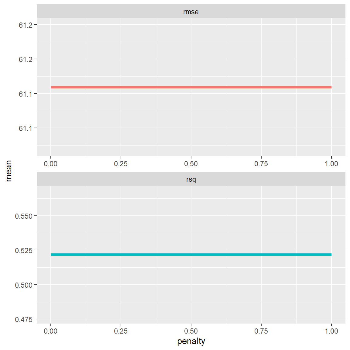

Hm, the tuning did not seem to have a large effect. But the maximum penalty value automatically chosen by the grid_regular function was only 1. Specify your own grid of parameter values and repeat steps 5 to 7 above.

penalty_grid <- tibble(penalty = seq(0, 250, length.out = 200))

penalty_grid <- tibble(penalty = seq(0, 250, length.out = 200))

# step 5
ridge_grid <-
  ridge_workflow %>% 
  tune_grid(resamples = airbnb_folds,
            grid = penalty_grid)

# step 6
collect_metrics(ridge_grid)

# A tibble: 400 x 7
   penalty .metric .estimator   mean     n std_err .config               
     <dbl> <chr>   <chr>       <dbl> <int>   <dbl> <chr>                 
 1    0    rmse    standard   61.1      10 19.7    Preprocessor1_Model001
 2    0    rsq     standard    0.522    10  0.0371 Preprocessor1_Model001
 3    1.26 rmse    standard   61.1      10 19.7    Preprocessor1_Model002
 4    1.26 rsq     standard    0.522    10  0.0371 Preprocessor1_Model002
 5    2.51 rmse    standard   61.1      10 19.7    Preprocessor1_Model003
 6    2.51 rsq     standard    0.522    10  0.0371 Preprocessor1_Model003
 7    3.77 rmse    standard   61.1      10 19.7    Preprocessor1_Model004
 8    3.77 rsq     standard    0.522    10  0.0371 Preprocessor1_Model004
 9    5.03 rmse    standard   61.2      10 19.8    Preprocessor1_Model005
10    5.03 rsq     standard    0.521    10  0.0371 Preprocessor1_Model005
# ... with 390 more rows

# step 7
ridge_grid %>%
  collect_metrics() %>%
  ggplot(aes(penalty, mean, color = .metric)) +
  geom_line(size = 1.5) +
  facet_wrap(~.metric, scales = "free", nrow = 2) +
  theme(legend.position = "none")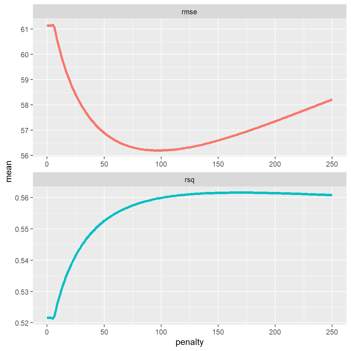

Now we see a drop in the RMSE at higher penalty values. Select the best penalty value by passing ridge_grid into the select_best() function and save the output as best_ridge.

XX <- XX(XX, "rmse")

best_ridge <- select_best(ridge_grid, "rmse")

Now let’s finalize our workflow using the finalize_workflow() function. Pass it the ridge_workflow and the best_ridge objects as first and second arguments. Save the output as final_ridge.

final_ridge <- 
  ridge_workflow %>% 
  finalize_workflow(best_ridge)

Now we can fit the model using the final workflow. Use the fit() function to this end, by passing it the final_ridge workflow and airbnb_train. Save the output as ridge_res.

ridge_res <- fit(final_ridge, airbnb_train)

Use the tidy() function to look at the parameter values of ridge_res.

tidy(ridge_res)

# A tibble: 35 x 3
   term                   estimate penalty
   <chr>                     <dbl>   <dbl>
 1 (Intercept)              69.9      96.7
 2 accommodates             19.7      96.7
 3 bedrooms                 13.0      96.7
 4 bathrooms                 7.47     96.7
 5 cleaning_fee              2.00     96.7
 6 availability_90_days      1.24     96.7
 7 host_response_rate       -0.479    96.7
 8 host_superhost            4.65     96.7
 9 host_listings_count       2.84     96.7
10 review_scores_accuracy    1.03     96.7
# ... with 25 more rows

The last_fit() function, which you can use with the final_ridge workflow instead of the fit() function, let’s you directly evaluate the model performance. Pass the final_ridge and airbnb_split (! instead of the airbnb_train) objects into last_fit() and directly pipe the output into collect_metrics().

XX(XX, XX) %>% 
  XX()

last_fit(final_ridge, airbnb_split) %>% 
  collect_metrics()

# A tibble: 2 x 4
  .metric .estimator .estimate .config             
  <chr>   <chr>          <dbl> <chr>               
1 rmse    standard      49.6   Preprocessor1_Model1
2 rsq     standard       0.465 Preprocessor1_Model1

F - Lasso Regression

Now it’s time to fit a lasso regression. We can use the ridge_recipe from before, so no need to specify a new recipe.

Create a lasso regression model, again using the linear_reg() model and the glmnet engine. Within linear_reg(), set the argument mixture to 1 and penalty to tune(). Save the output as lasso_model

# set up the lasso regression model
XX <- 
  XX(XX = XX, XX = XX) %>% 
  set_engine(XX) %>% 
  set_mode("regression")

# set up the lasso regression model
lasso_model <- 
  linear_reg(mixture = 1, penalty = tune()) %>% 
  set_engine("glmnet") %>% 
  set_mode("regression")

Create a workflow called lasso_workflow using workflow() and add the ridge_recipe and lasso_model objects.

# lasso workflow 
lasso_workflow <- 
  workflow() %>% 
  add_recipe(ridge_recipe) %>% 
  add_model(lasso_model)

Set up a grid of tuning parameters. Here we will directly specify our own grid. We’ll use the same as with the ridge regression:

penalty_grid <- tibble(penalty = seq(0, 25, length.out = 200))

penalty_grid <- tibble(penalty = seq(0, 25, length.out = 200))

Tune the model on the training data. To do so using our resampling scheme, use the tune_grid() function instead of the fit() or fit_resamples() function. Pass it the defined workflow as first argument and set the resamples argument to airbnb_folds, and the grid argument to penalty_grid. Save the output as lasso_grid.

# tune the penalty parameter
lasso_grid <-
  lasso_workflow %>% 
  tune_grid(resamples = airbnb_folds,
            grid = penalty_grid)

Use collect_metrics() to evaluate the cross-validation performance of the model across the different values of the penalty parameter.

collect_metrics(lasso_grid)

# A tibble: 400 x 7
   penalty .metric .estimator   mean     n std_err .config               
     <dbl> <chr>   <chr>       <dbl> <int>   <dbl> <chr>                 
 1   0     rmse    standard   62.7      10 19.4    Preprocessor1_Model001
 2   0     rsq     standard    0.511    10  0.0392 Preprocessor1_Model001
 3   0.126 rmse    standard   62.5      10 19.5    Preprocessor1_Model002
 4   0.126 rsq     standard    0.512    10  0.0392 Preprocessor1_Model002
 5   0.251 rmse    standard   62.2      10 19.5    Preprocessor1_Model003
 6   0.251 rsq     standard    0.514    10  0.0390 Preprocessor1_Model003
 7   0.377 rmse    standard   62.0      10 19.5    Preprocessor1_Model004
 8   0.377 rsq     standard    0.516    10  0.0389 Preprocessor1_Model004
 9   0.503 rmse    standard   61.8      10 19.6    Preprocessor1_Model005
10   0.503 rsq     standard    0.518    10  0.0387 Preprocessor1_Model005
# ... with 390 more rows

Plot the penalty value on the x axis, and the performance metrics on the y axis. Use the code below to do so.

lasso_grid %>%
  collect_metrics() %>%
  ggplot(aes(penalty, mean, color = .metric)) +
  geom_line(size = 1.5) +
  facet_wrap(~.metric, scales = "free", nrow = 2) +
  theme(legend.position = "none")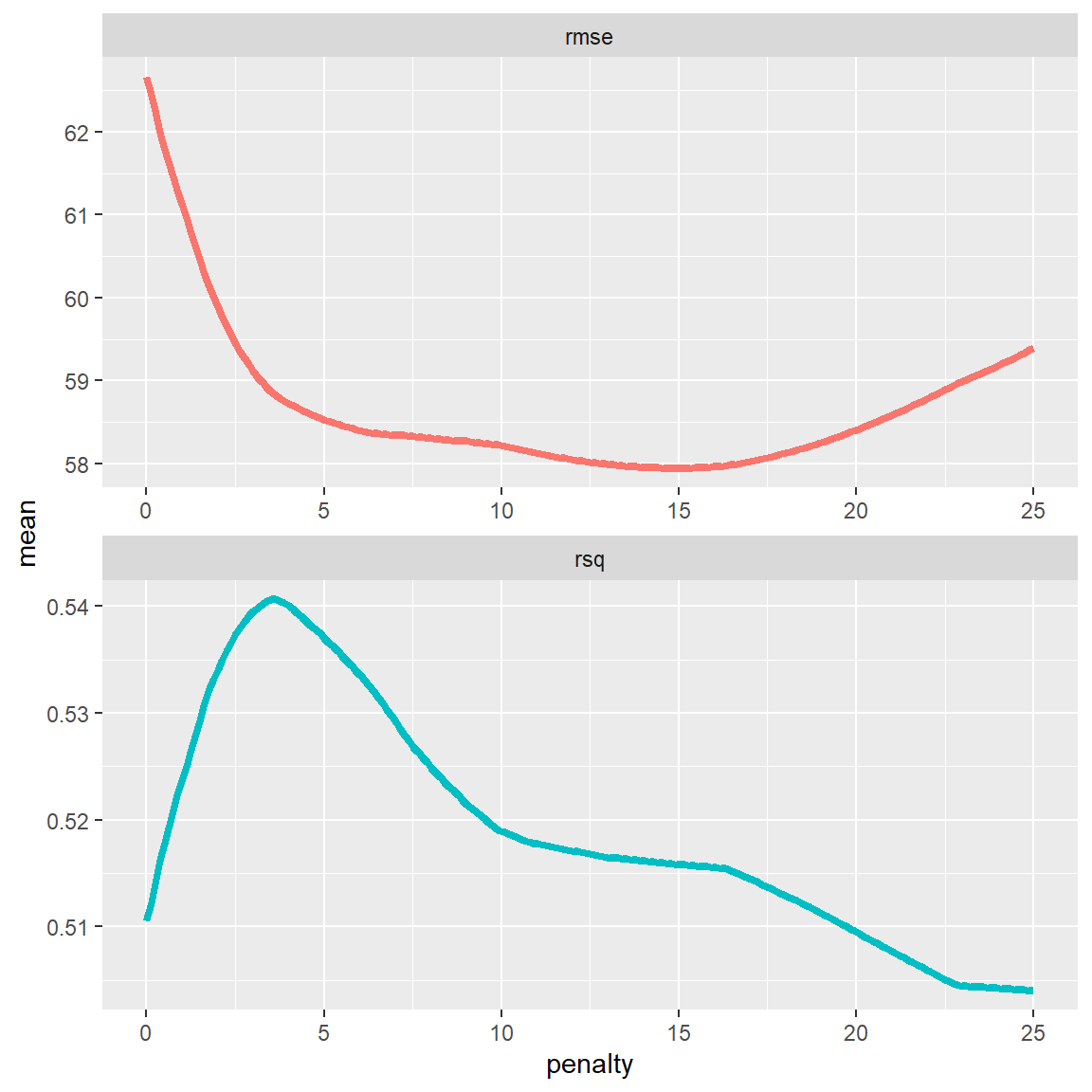

Select the best penalty value by passing lasso_grid into the select_best() function and save the output as best_lasso.

XX <- XX(XX, "rmse")

best_lasso <- select_best(lasso_grid, "rmse")

Finalize the workflow using the finalize_workflow() function. Pass it the lasso_workflow and the best_lasso objects as first and second arguments. Save the output as final_lasso.

final_lasso <- 
  lasso_workflow %>% 
  finalize_workflow(best_lasso)

Fit the model using the final workflow. Use the fit() function to this end, by passing it the final_lasso workflow and airbnb_train. Save the output as lasso_res.

lasso_res <- fit(final_lasso, airbnb_train)

Use the tidy() function to look at the parameter values of lasso_res. Which variables are important and which were set to 0?

tidy(lasso_res)

# A tibble: 35 x 3
   term                   estimate penalty
   <chr>                     <dbl>   <dbl>
 1 (Intercept)               71.7     14.8
 2 accommodates              37.5     14.8
 3 bedrooms                   4.56    14.8
 4 bathrooms                  0       14.8
 5 cleaning_fee               0       14.8
 6 availability_90_days       0       14.8
 7 host_response_rate         0       14.8
 8 host_superhost             0       14.8
 9 host_listings_count        0       14.8
10 review_scores_accuracy     0       14.8
# ... with 25 more rows

G - Decision Tree

It’s time to fit an optimized decision tree model!

Decision trees don’t need categorical variables to be dummy coded. Create a new recipe called tree_recipe that uses all available predictors to predict the price of Airbnbs based on the airbnb_train data. In addition, use the pre-proccessing step step_other(all_nominal_predictors(), threshold = 0.005). This will lump together all cases of categorical variables that make up less than 0.5% of the cases into an other category. This will prevent issues when assessing performance using the test set.

tree_recipe <-
  recipe(price ~ ., data = airbnb_train) %>% 
  step_other(all_nominal_predictors(), threshold = 0.005)

Set up a decision tree model. Use the decision_tree() function to specify the model, and set the engine to rpart. Set the mode to "regression". Call the output dt_model. Within decision_tree() specify the argument cost_complexity = tune().

# set up the decision tree model
dt_model <- 
  decision_tree(cost_complexity = tune()) %>% 
  set_engine("rpart") %>% 
  set_mode("regression")

Create a new workflow dt_workflow, where you add the newly created tree_recipe and the dt_model.

# decision tree workflow  
dt_workflow <- 
  workflow() %>% 
  add_recipe(tree_recipe) %>% 
  add_model(dt_model)

Set up a grid of tuning parameters. Use the following code to do so:

complexity_grid <- tibble(cost_complexity =  seq(from = 0, to = .01, length = 100))

Tune the model on the training data. To do so using our resampling scheme, use the tune_grid() function and pass it the defined workflow as first argument and set the resamples argument to airbnb_folds, and the grid argument to complexity_grid. Save the output as dt_grid. (Note: This will take some time…)

# tune the cost complexity parameter
dt_grid <-
  dt_workflow %>% 
  tune_grid(resamples = airbnb_folds,
            grid = complexity_grid)

Plot the cost_complexity value on the x axis, and the performance metrics on the y axis. Use the code below to do so.

dt_grid %>%
  collect_metrics() %>%
  ggplot(aes(cost_complexity, mean, color = .metric)) +
  geom_line(size = 1.5) +
  facet_wrap(~.metric, scales = "free", nrow = 2) +
  theme(legend.position = "none")

Select the best cost_complexity value by passing dt_grid into the select_best() function and save the output as best_dt.

XX <- XX(XX, "rmse")

best_dt <- select_best(dt_grid, "rmse")

Finalize the workflow using the finalize_workflow() function. Pass it the dt_workflow and the best_dt objects as first and second arguments. Save the output as final_dt.

final_dt <- 
  dt_workflow %>% 
  finalize_workflow(best_dt)

Fit the model using the final workflow. Use the fit() function to this end, by passing it the final_dt workflow and airbnb_train. Save the output as dt_res.

dt_res <- fit(final_dt, airbnb_train)

H - Random Forests

It’s time to fit an optimized random forest model!

As random forests are made up of many decision trees, we can use the recipe we defined for the decision tree, so we only have to set up a random forest model. Use the rand_forest() function to specify the model, and set the engine to "ranger". Set the mode to "regression". Call the output rf_model. In the rand_forest() function, set the mtry argument to tune().

# set up the random forest model
rf_model <- 
  rand_forest(mtry = tune()) %>% 
  set_engine("ranger") %>% 
  set_mode("regression")

Create a new workflow rf_workflow, where you add the tree_recipe and the newly created rf_model.

# random forest workflow  
rf_workflow <- 
  workflow() %>% 
  add_recipe(tree_recipe) %>% 
  add_model(rf_model)

Set up a grid of tuning parameters. Use the following code to do so:

mtry_grid <- tibble(mtry = 1:15)

Tune the model on the training data. To do so using our resampling scheme, use the tune_grid() function and pass it the defined workflow as first argument and set the resamples argument to airbnb_folds, and the grid argument to mtry_grid. Save the output as rf_grid. (Note: This will again take some time… Actually even some more… Welcome in the world of machine learning…)

# tune the mtry parameter
rf_grid <-
  rf_workflow %>% 
  tune_grid(resamples = airbnb_folds,
            grid = mtry_grid)

Plot the mtry value on the x axis, and the performance metrics on the y axis. Use the code below to do so.

rf_grid %>%
  collect_metrics() %>%
  ggplot(aes(mtry, mean, color = .metric)) +
  geom_line(size = 1.5) +
  facet_wrap(~.metric, scales = "free", nrow = 2) +
  theme(legend.position = "none")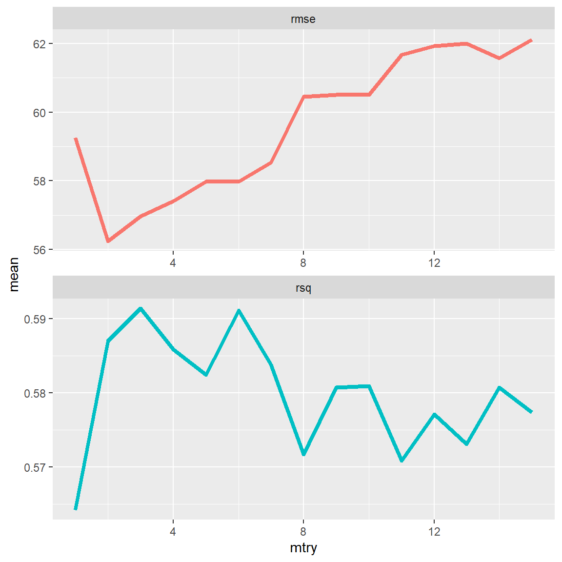

Select the best mtry value by passing rf_grid into the select_best() function and save the output as best_rf.

best_rf <- select_best(rf_grid, "rmse")

Finalize the workflow using the finalize_workflow() function. Pass it the rf_workflow and the best_rf objects as first and second arguments. Save the output as final_rf.

final_rf <- 
  rf_workflow %>% 
  finalize_workflow(best_rf)

Fit the model using the final workflow. Use the fit() function to this end, by passing it the final_rf workflow and airbnb_train. Save the output as rf_res.

rf_res <- fit(final_rf, airbnb_train)

I - Estimate prediction accuracy from training folds

Using the following code as template, evaluate and compare the model performances of the different models.

XX_res %>% 
  predict(new_data = airbnb_train) %>% 
  bind_cols(airbnb_train %>% select(price)) %>% 
  metrics(truth = price, estimate = .pred)

lm_res %>% 
  predict(new_data = airbnb_train) %>% 
  bind_cols(airbnb_train %>% select(price)) %>% 
  metrics(truth = price, estimate = .pred)

# A tibble: 3 x 3
  .metric .estimator .estimate
  <chr>   <chr>          <dbl>
1 rmse    standard      77.3  
2 rsq     standard       0.370
3 mae     standard      31.1

ridge_res %>% 
  predict(new_data = airbnb_train) %>% 
  bind_cols(airbnb_train %>% select(price)) %>% 
  metrics(truth = price, estimate = .pred)

# A tibble: 3 x 3
  .metric .estimator .estimate
  <chr>   <chr>          <dbl>
1 rmse    standard      80.8  
2 rsq     standard       0.344
3 mae     standard      26.5

lasso_res %>% 
  predict(new_data = airbnb_train) %>% 
  bind_cols(airbnb_train %>% select(price)) %>% 
  metrics(truth = price, estimate = .pred)

# A tibble: 3 x 3
  .metric .estimator .estimate
  <chr>   <chr>          <dbl>
1 rmse    standard      81.1  
2 rsq     standard       0.331
3 mae     standard      27.4

dt_res %>% 
  predict(new_data = airbnb_train) %>% 
  bind_cols(airbnb_train %>% select(price)) %>% 
  metrics(truth = price, estimate = .pred)

# A tibble: 3 x 3
  .metric .estimator .estimate
  <chr>   <chr>          <dbl>
1 rmse    standard      77.3  
2 rsq     standard       0.370
3 mae     standard      25.0

rf_res %>% 
  predict(new_data = airbnb_train) %>% 
  bind_cols(airbnb_train %>% select(price)) %>% 
  metrics(truth = price, estimate = .pred)

# A tibble: 3 x 3
  .metric .estimator .estimate
  <chr>   <chr>          <dbl>
1 rmse    standard      51.8  
2 rsq     standard       0.820
3 mae     standard      16.9

J - Calculate prediction accuracy

Now, based on the same template, but this time using the test data, evaluate and compare the out-of-sample model performances.

lm_res %>% 
  predict(new_data = airbnb_test) %>% 
  bind_cols(airbnb_test %>% select(price)) %>% 
  metrics(truth = price, estimate = .pred)

# A tibble: 3 x 3
  .metric .estimator .estimate
  <chr>   <chr>          <dbl>
1 rmse    standard      48.7  
2 rsq     standard       0.485
3 mae     standard      29.9

ridge_res %>% 
  predict(new_data = airbnb_test) %>% 
  bind_cols(airbnb_test %>% select(price)) %>% 
  metrics(truth = price, estimate = .pred)

# A tibble: 3 x 3
  .metric .estimator .estimate
  <chr>   <chr>          <dbl>
1 rmse    standard      49.6  
2 rsq     standard       0.465
3 mae     standard      24.0

lasso_res %>% 
  predict(new_data = airbnb_test) %>% 
  bind_cols(airbnb_test %>% select(price)) %>% 
  metrics(truth = price, estimate = .pred)

# A tibble: 3 x 3
  .metric .estimator .estimate
  <chr>   <chr>          <dbl>
1 rmse    standard      50.0  
2 rsq     standard       0.443
3 mae     standard      26.1

dt_res %>% 
  predict(new_data = airbnb_test) %>% 
  bind_cols(airbnb_test %>% select(price)) %>% 
  metrics(truth = price, estimate = .pred)

# A tibble: 3 x 3
  .metric .estimator .estimate
  <chr>   <chr>          <dbl>
1 rmse    standard      42.0  
2 rsq     standard       0.610
3 mae     standard      24.4

rf_res %>% 
  predict(new_data = airbnb_test) %>% 
  bind_cols(airbnb_test %>% select(price)) %>% 
  metrics(truth = price, estimate = .pred)

# A tibble: 3 x 3
  .metric .estimator .estimate
  <chr>   <chr>          <dbl>
1 rmse    standard      27.7  
2 rsq     standard       0.840
3 mae     standard      20.0

Which of your models had the best performance in the true test data?
How close were your models’ true prediction error to the values you estimated in the previous section based on the training data?

Examples

# Fitting and evaluating a regression model ------------------------------------

# Step 0: Load packages---------------------------------------------------------
library(tidyverse)    # Load tidyverse for dplyr and tidyr
library(tidymodels)   # For ML mastery 
tidymodels_prefer()   # To resolve common conflicts

# Step 1: Load and Clean, and Explore Training data ----------------------------

# I'll use the mpg dataset from the dplyr package 
# Explore training data
mpg        # Print the dataset
View(mpg)  # Open in a new spreadsheet-like window 
dim(mpg)   # Print dimensions
names(mpg) # Print the names

# Step 2: Split the data--------------------------------------------------------

mpg_split <- initial_split(mpg)
data_train <- training(mpg_split)
data_test <- testing(mpg_split)

# Step 3: Define resampling scheme ---------------------------------------------

# Use 10-fold cross validation
data_folds <- vfold_cv(data_train, v = 10) 

# Step 4: Define recipe --------------------------------------------------------

# The recipe defines what to predict with what, and how to pre-process the data
lasso_recipe <- 
  recipe(hwy ~ year + cyl + displ + trans,  # Specify formula
         data = data_train) %>%             # Specify the data
  step_dummy(all_nominal_predictors()) %>%  # Dummy code all categorical predictors
  step_normalize(all_numeric_predictors())  # Center and scale numeric variables


# Step 5: Define model ---------------------------------------------------------

# The model definition defines what kind of model we want to use and how to
# fit it
lasso_model <- 
  linear_reg(mixture = 1,           # Specify model type and parameters
             penalty = tune()) %>%        
  set_engine("glmnet") %>%          # Specify engine (often package name) to use
  set_mode("regression")            # Specify whether it's a regressio or 
                                    # classification problem.

# Step 6: Define workflow ------------------------------------------------------

# The workflow combines model and recipe, so that we can fit the model
lasso_workflow <- 
  workflow() %>%                # Initialize workflow
  add_model(lasso_model) %>%    # Add the model to the workflow
  add_recipe(lasso_recipe)      # Add the recipe to the workflow

# Step 7: Tune parameters ------------------------------------------------------

# Create a grid of parameter values to test
penalty_grid <- tibble(penalty = 10 ^ (seq(-4, 5, length = 150)))

# tune the penalty parameter
lasso_grid <-
  lasso_workflow %>%                 # The workflow
  tune_grid(resamples = data_folds,  # The resampling scheme
            grid = penalty_grid)     # The parameter grid

# Step 8: Finalize workflow ----------------------------------------------------

# Select best parameter values
best_lasso <- select_best(lasso_grid, "rmse")

# finalise workflow
final_lasso <- 
  lasso_workflow %>% 
  finalize_workflow(best_lasso)

# Step 9: Fit model based on best hyper-parameter ------------------------------

# Fit the model on complete training data, using the best hyper-parameter value
lasso_res <- fit(final_lasso, data_train) 

# Look at summary information
tidy(lasso_res)        

# Step 10: Assess prediction performance ----------------------------------------
# Save model predictions and observed values
lasso_pred <- 
  lasso_res %>%            # Model from which to extract predictions
  predict(data_test) %>%   # Obtain predictions, based on entered data (in this
                           #  case, these predictions ARE out-of-sample)
  bind_cols(data_test %>% select(hwy))  # Extract observed/true values

# Obtain performance metrics
metrics(lasso_pred, truth = hwy, estimate = .pred)

Datasets

The dataset contains data of the 1191 apartments that were added on Airbnb for the Berlin area in the year 2018.

File	Rows	Columns
airbnb.csv	1191	23

Variable description of `airbnb`

Name	Description
price	Price per night (in $s)
accommodates	Number of people the airbnb accommodates
bedrooms	Number of bedrooms
bathrooms	Number of bathrooms
cleaning_fee	Amount of cleaning fee (in $s)
availability_90_days	How many of the following 90 days the airbnb is available
district	The district the Airbnb is located in
host_respons_time	Host average response time
host_response_rate	Host response rate
host_superhost	Whether host is a superhost TRUE/FALSE
host_listings_count	Number of listings the host has
review_scores_accuracy	Accuracy of information rating [0, 10]
review_scores_cleanliness	Cleanliness rating [0, 10]
review_scores_checkin	Check in rating [0, 10]
review_scores_communication	Communication rating [0, 10]
review_scores_location	Location rating [0, 10]
review_scores_value	Value rating [0, 10]
kitchen	Kitchen available TRUE/FALSE
tv	TV available TRUE/FALSE
coffe_machine	Coffee machine available TRUE/FALSE
dishwasher	Dishwasher available TRUE/FALSE
terrace	Terrace/balcony available TRUE/FALSE
bathtub	Bathtub available TRUE/FALSE

Functions

Packages

Package	Installation
`tidyverse`	`install.packages("tidyverse")`
`tidymodels`	`install.packages("tidymodels")`
`rpart.plot`	`install.packages("rpart.plot")`

Functions

Resources

tidymodels webpage: Can be used as cheat sheet. Also has some tutorials.
The, not yet completed, book Tidymodeling with R: More detailed introduction into the tidymodels framework.

Tuning

Applied Machine Learning with R The R Bootcamp @ AMLD

Overview

Tasks

A - Setup

B - Data splitting

C - Setup resampling scheme

D - Regression (standard)

E - Ridge Regression

F - Lasso Regression

G - Decision Tree

H - Random Forests

I - Estimate prediction accuracy from training folds

J - Calculate prediction accuracy

Examples

Datasets

Variable description of airbnb

Functions

Packages

Functions

Resources

Applied Machine Learning with R
The R Bootcamp @ AMLD

Variable description of `airbnb`