Unsupervised learning

Overview

In this practical, you will learn how to apply cluster analysis to two data sets.

In the end, you will know how to:

How to identify clusterings using different algorithms.
How to estimate the number of clusters for a given problem.

Tasks

A - Setup

Open your TheRBootcamp R project.
Open a new R script. Write your name, the date and “Unsupervised learning Practical” as comments at the top.

## NAME
## DATUM
## Unsupervised learning practical

Save the script as Unsupervised_practical.R in the 2_Code folder.
Load the packages tidyverse, cstab, dbscan, and mclust.

B - Load the `gap` data set

Using read_csv(), read in gap.csv and save it as gap.

# Read gap.csv
gap <- read_csv('1_Data/gap.csv')

Print the data set and inspect its contents.
Use summary() to get additional insight into the data.
Use the code below to create a new data set containing only the data from year 2007 and features Lebenserwartung and BIP pro Kopf.

# gap in 2007
gap2007 <- gap %>% 
  filter(Jahr == 2007) %>% 
  select(`BIP pro Kopf`, Lebenserwartung)

C - k-means

Using kmeans(), identify three clusters (centers) in gap2007.

# kmeans of gap in 2007
gap2007_km <- kmeans(x = XX, centers = XX)

# kmeans of gap in 2007
gap2007_km <- kmeans(x = gap2007, centers = 3)

Print gap2007_km and study the output.

# kmeans of gap in 2007
gap2007_km

K-means clustering with 3 clusters of sizes 27, 80, 34

Cluster means:
  BIP pro Kopf Lebenserwartung
1        34099            79.9
2         2809            60.3
3        13701            72.1

Clustering vector:
  [1] 2 2 2 2 3 1 1 1 2 1 2 2 2 3 3 3 2 2 2 2 1 2 2 3 2 2 2 2 2 3 2 3 3 3 1 2 2
 [38] 2 2 2 3 2 2 1 1 3 2 1 2 1 2 2 2 2 2 1 3 1 2 2 3 2 1 1 1 2 1 2 2 2 3 3 2 2
 [75] 3 2 2 3 2 2 3 3 2 3 2 2 2 2 2 1 1 2 2 2 1 3 2 3 2 2 2 3 3 3 2 3 2 2 3 2 3
[112] 2 1 3 1 2 3 1 2 2 2 1 1 2 1 2 2 2 3 2 3 2 1 1 3 3 2 2 2 2 2

Within cluster sum of squares by cluster:
[1] 9.86e+08 3.76e+08 6.82e+08
 (between_SS / total_SS =  90.7 %)

Available components:

[1] "cluster"      "centers"      "totss"        "withinss"     "tot.withinss"
[6] "betweenss"    "size"         "iter"         "ifault"

The first row of the output and the table Cluster means shows how many objects were assigned to each of the three clusters and where the centroids (cluster means) of these are located.
At the bottom of the output is a list of names of objects contained in the clustering object. Use gap2007_km$XX to select the object clusters, as well as the elements centers and store them as clusters and centers respectively.

# gap2007_km 
clusters <- gap2007_km$XX
centers <- gap2007_km$XX

# gap2007_km 
clusters <- gap2007_km$cluster
centers <- gap2007_km$centers

Use the code below to plot the data and cluster assignments.

# kmeans of gap in 2007
plot(gap2007, col = clusters)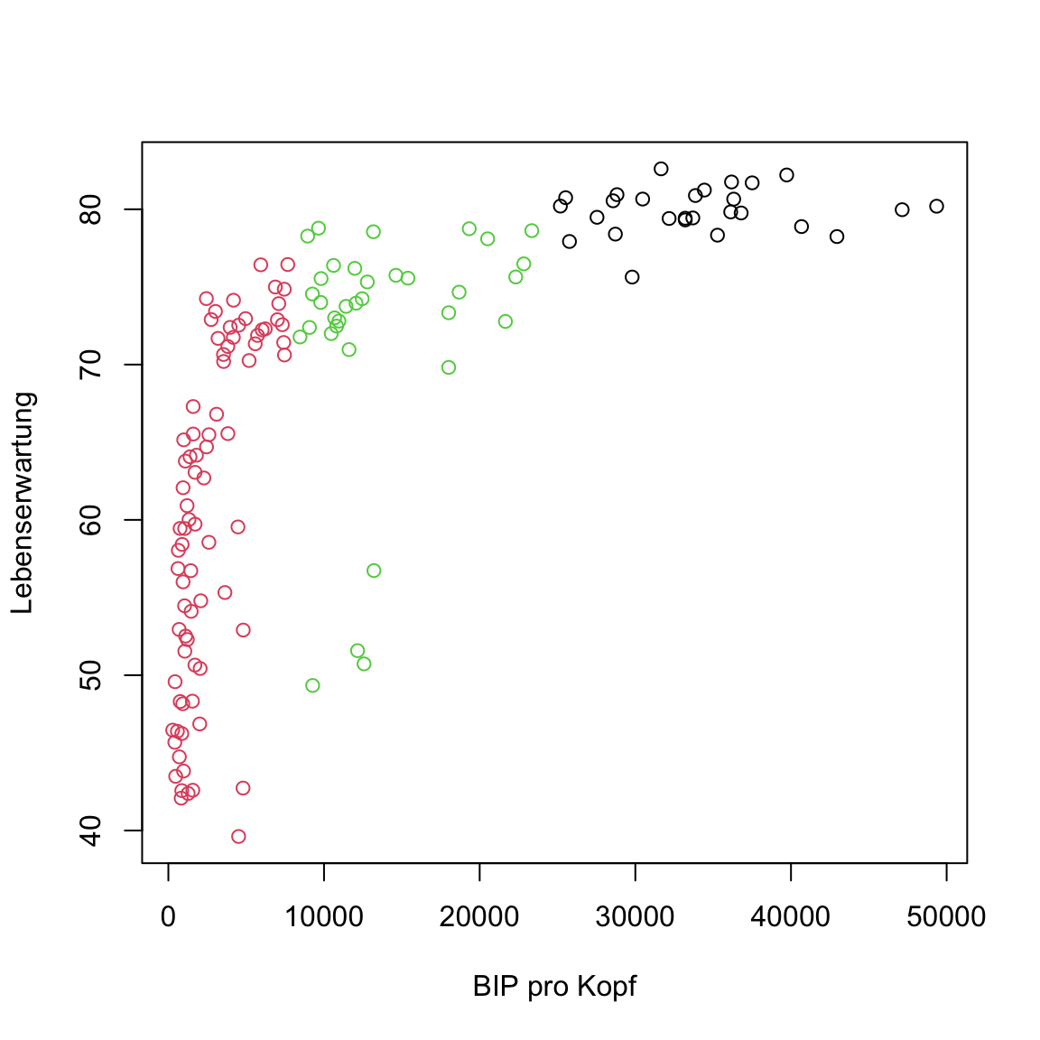

Now use the code below to add the centroids.

# kmeans of gap in 2007
plot(gap2007, col = clusters)
points(centers, pch = 16, col = 1:3, cex = 2)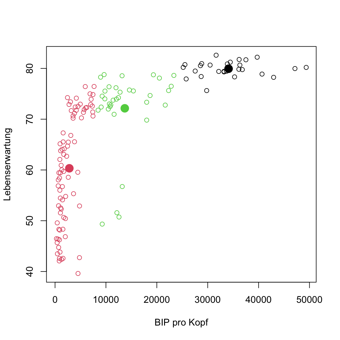

Something’s off, right? Some points of the middle cluster actually seem to lie closer to the bottom-left cluster. This shouldn’t be the case. Any ideas how this has come about?
The problem is that the features have different scales. The values of BIP pro Kopf are way larger than those in Lebenserwartung and, thus, a lot further away from each other. For that reason, BIP pro Kopf plays a much larger role for cluster assignments than Lebenserwartung. To fix this problem, run the code below, which scaled the features in gap2007.

# scale gap in 2007
gap2007_scaled <- gap2007 %>% 
  scale() %>% 
  as_tibble()

Now, run kmeans() for gap2007_scaled and plot the data and cluster assignments. All good now?

# kmeans plot for gap in 2007 
gap2007_scaled_km <- kmeans(x = gap2007_scaled, centers = 3) 

# extract elements
clusters <- gap2007_scaled_km$cluster
centers <- gap2007_scaled_km$centers

# plot
plot(gap2007_scaled, col = clusters)
points(centers, pch = 16, col = 1:3, cex = 2)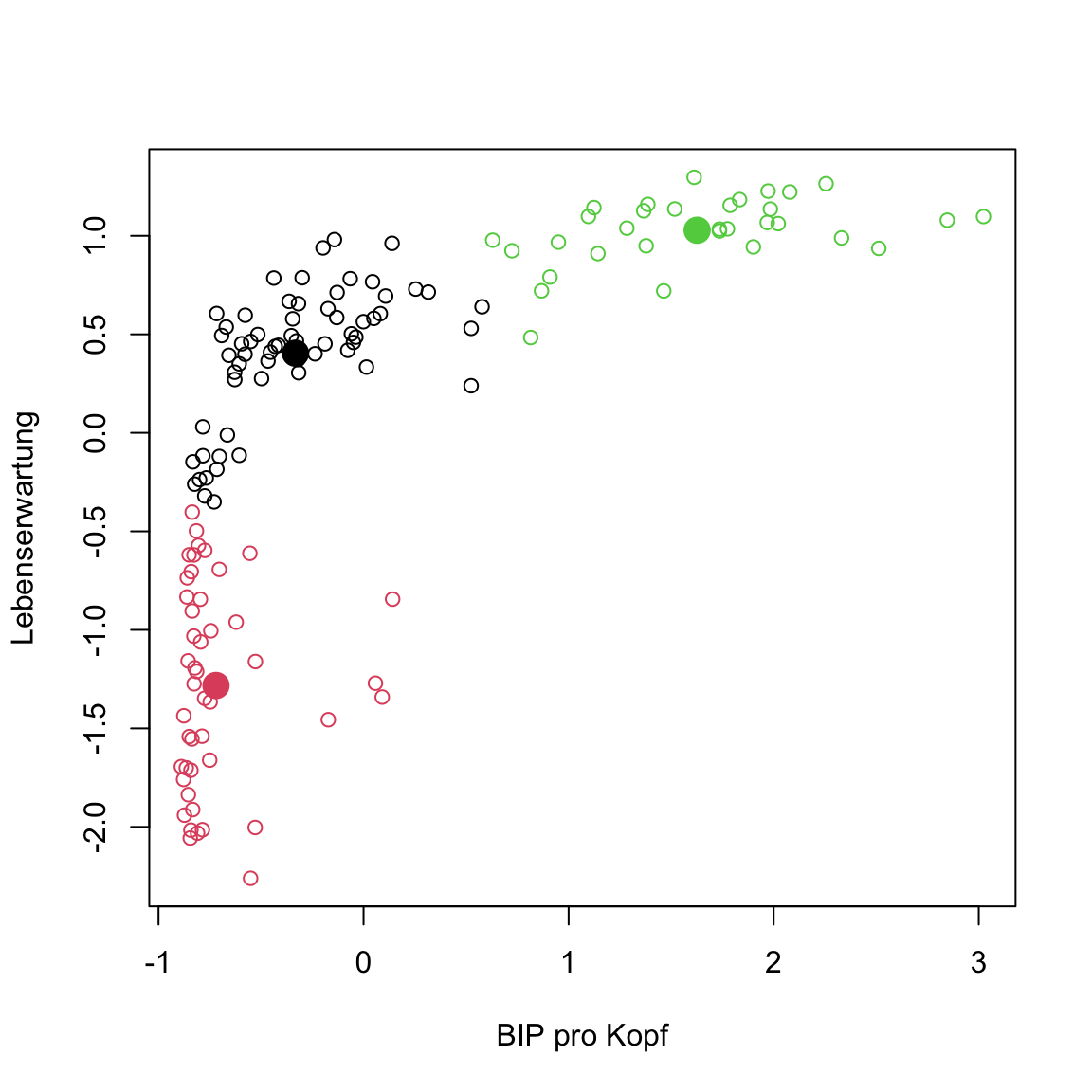

D - k-selection

It’s time to estimate how many clusters there might be in the data. Use the code below to create a vector of within-cluster variances for kmeans solutions associated with 2 to 20 clusters. The code uses the gap2007_scaled data.

# within-cluster variance development
km_development <- purrr::map(2:20, kmeans, x = gap2007_scaled)
withinvar <- purrr::map_dbl(km_development, 
                            `[[`, i = 'tot.withinss')

Using plot() create a plot of the development of the withinvar.

# kmeans within-variance development
plot(withinvar)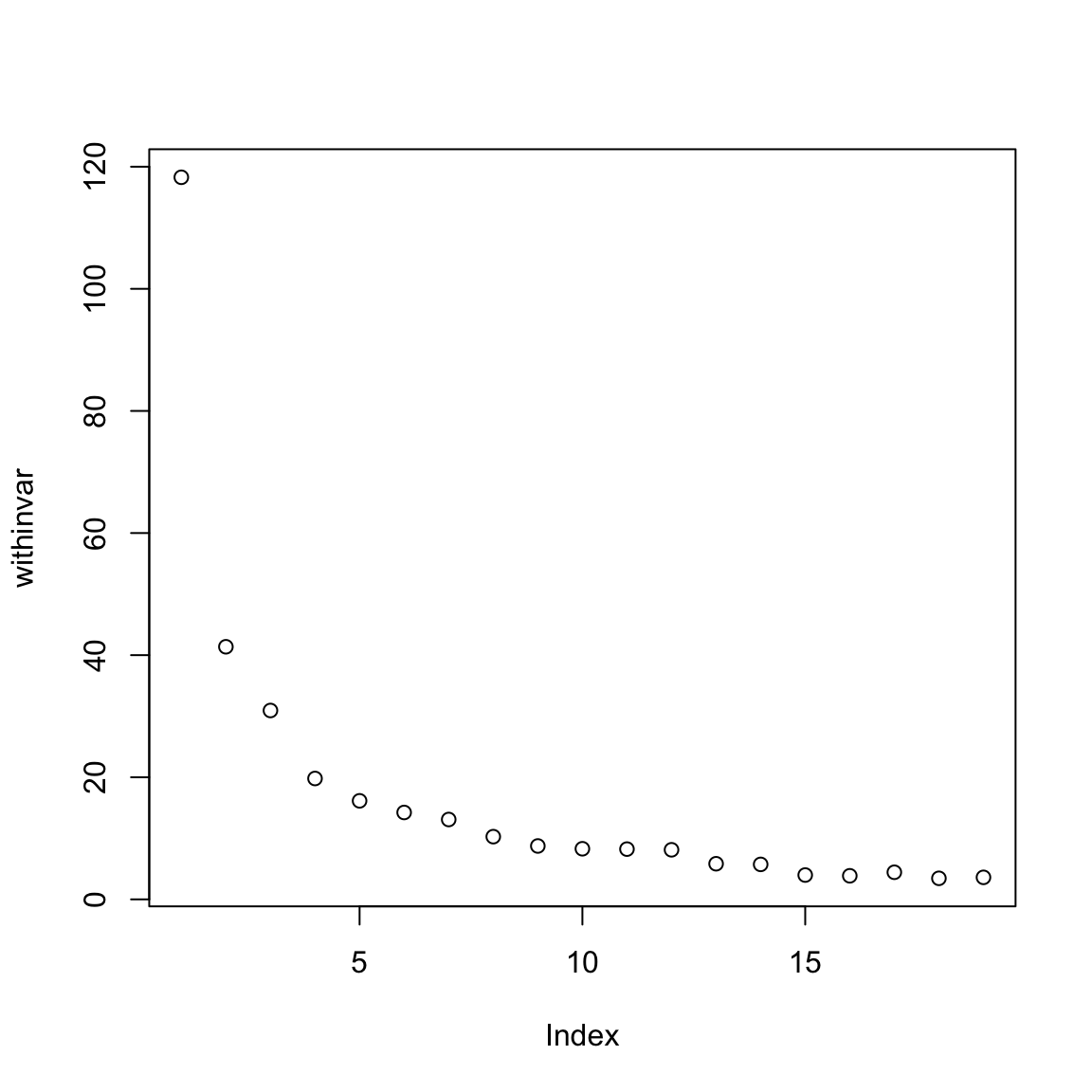

What does the plot tell you? Is there an elbow that would suggest a particular value of k?
Several values of k seem plausible: 1, 3, or 7. Use cDistance() from the cstab package to estimate k with values from 2 to 20 (2:20) as candidates.

# estimate k with cstab
k_est <- cDistance(data = as.matrix(XX),
                   kseq = XX:XX)

# estimate k with cstab
k_est <- cDistance(data = as.matrix(gap2007_scaled),
                   kseq = 2:20)

Extract k_est$k_Gap und k_est$k_Slope. Do the numbers seem reasonable?

# estimate k with cstab
k_est$k_Gap

[1] 14

k_est$k_Slope

[1] 3

Now try cStability() and extract k_instab. Reasonable?

# estimate k with cstab
k_est <- cStability(data = as.matrix(gap2007_scaled),
                   kseq = 2:20)



========
================
========================
================================
========================================
================================================
========================================================
================================================================
========================================================================
================================================================================

k_est$k_instab

[1] 3

Remember: There is no true k.

E - DBSCAN

Use dbscan() from the dbscan package to cluster the data. Again it is essential to work with gap2007_scaled as otherwise eps would describe an ellipse and not a circle. Set eps to .5.

# cluster using DBSCAN
gap2007_scaled_dbscan <- dbscan(x = XX, 
                                eps = XX)

# cluster using DBSCAN
gap2007_scaled_dbscan <- dbscan(x = gap2007_scaled, 
                                eps = .5)

Print gap2007_scaled_dbscan. What does the outpute tell you? Remember 0 means outlier.
A single cluster and 5 outliers were identified. Visualize the solution using the same approach as above. The + 1 is necessary as 0 implies no color.

# extract clusters
clusters <- gap2007_scaled_dbscan$XX

# plot
plot(XX, col = XX + 1)

# extract clusters
clusters <- gap2007_scaled_dbscan$cluster

# plot
plot(gap2007_scaled, col = clusters + 1)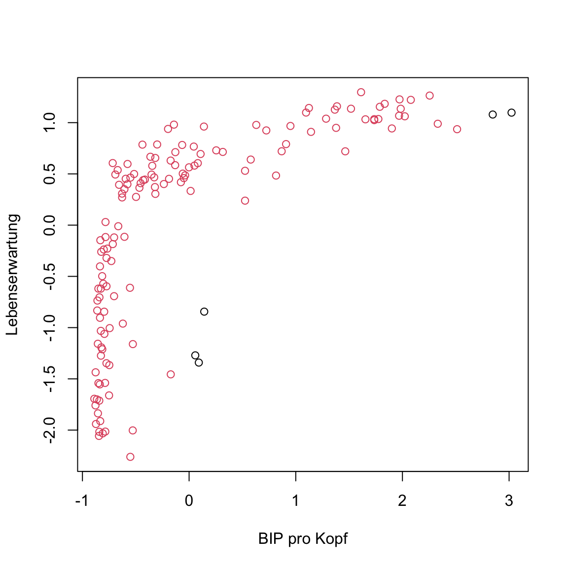

Now run dbscan() again using different values for eps. Try eps = .3 and eps = .1. Both times plot the results the same way as before. Any changes? Any of the solutions reasonable?

# cluster using DBSCAN
gap2007_scaled_dbscan.3 <- dbscan(x = gap2007_scaled, eps = .3)
gap2007_scaled_dbscan.1 <- dbscan(x = gap2007_scaled, eps = .1)

# plot
par(mfrow = c(1, 3))
plot(gap2007_scaled, col = gap2007_scaled_dbscan$cluster + 1)
plot(gap2007_scaled, col = gap2007_scaled_dbscan.3$cluster + 1)
plot(gap2007_scaled, col = gap2007_scaled_dbscan.1$cluster + 1)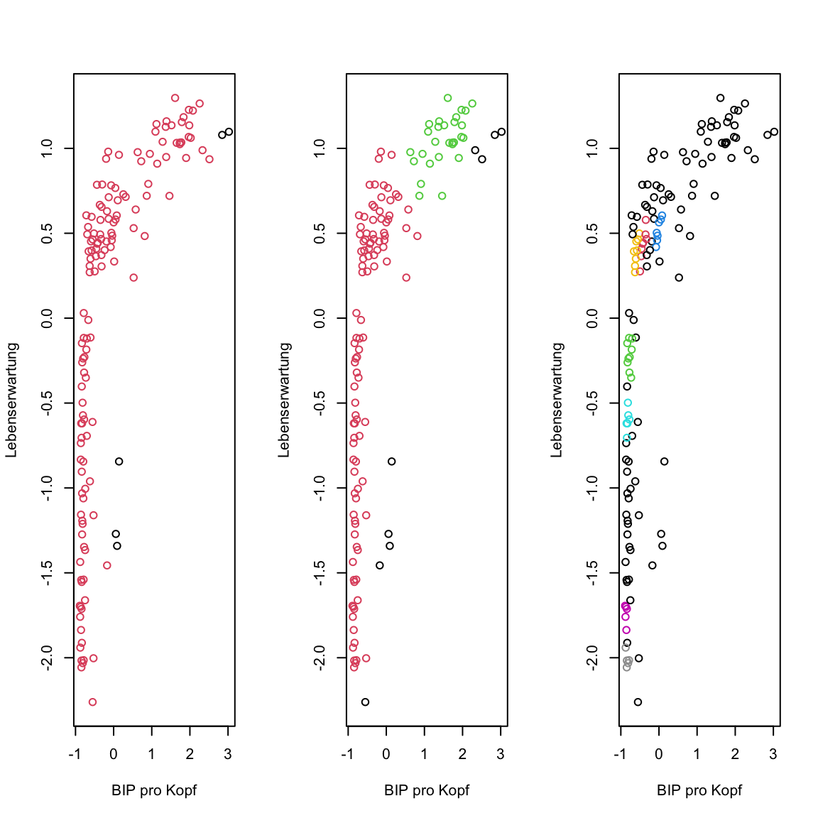

dbscan() has additional parameters. minPts determines the number of points within eps necessary for a point to be a core point. If you like, try different values to explore the effect of minPts.

F - Gaussian Mixtures

Finally, use Mclust from the mclust package to cluster the date using Gaussian mixtures. This time, you can work with the original data set gap2007 as Gaussian mixtures are able to account for the differences in scale.

# Gaussian mixtures
gap2007_gm <- Mclust(XX)

# Gaussian mixtures
gap2007_gm <- Mclust(gap2007)

Print the object gap2007_gm. What do you see?
The output of gap2007_gm reveals very little. It only shows which objects it contains. Use table(gap2007_gm$classification) to gain an overview over the cluster assignments. How many clusters were identified and how many does each contain?
Use the classification element to create a visualization of the cluster assignments.

# plot
plot(gap2007_scaled, col = gap2007_gm$classification)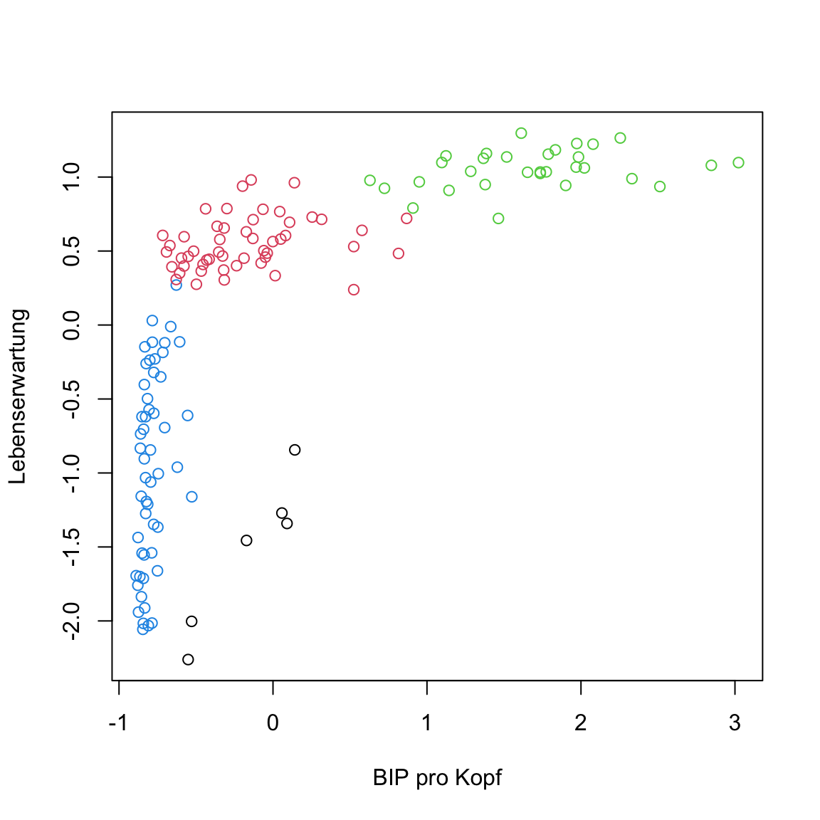

Now use `plot(gap2007_gm, what = 'classification') to create mclust’s own visualization.

# plot using mclust
plot(gap2007_gm, what = 'classification')

Try to understand what the ellipses in the mclust plot reveal about the clusters. Remember they represent normal distributions with variances and co-variances reflecting the correlations between the features.
One desirable property of Gaussian mixtures is that they produce estimates of the uncertainty associated with assigning a data point to a particular cluster. Use plot(gap2007_gm, what = 'uncertainty') to visualize this. The size of the points reflects the degree of uncertainty associated with a point being assigned to one particular cluster and not the others.

# plot
plot(gap2007_gm, what = 'uncertainty')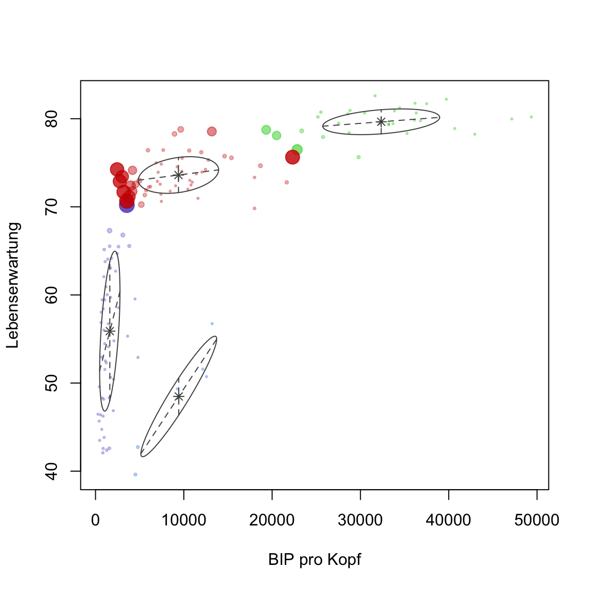

X - Challenges: Modellselection

A further useful property of Gaussian mixtures is the existence of different implementations with different complexity. In fact, Mclust() already considers a variety of implementations in addition to different values of k. You can gain an overview on the performance of these using plot(gap2007_gm, what = 'BIC').

# plot
plot(gap2007_gm, what = 'BIC')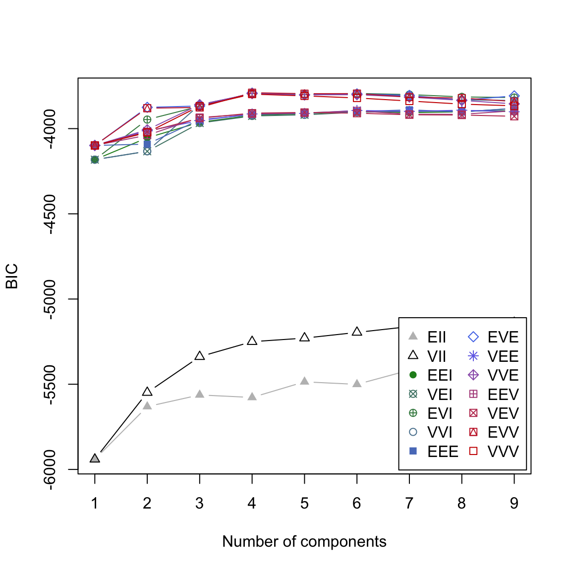

BIC is the Bayesian Information Criterion and it characterizes the model fit in relation to model complexity. In this case, higher BIC values indicate better performance. In the visualization you see the performance of 14 different implementations as a function of different values k (x-axis).

Use plot(gap2007_gm, what = 'BIC', ylim = c(-4200, -3900)) to get a better view on the critical region of the plot. Now you should be able to see that EVV for k=4 shows the best performance overall.

# plot
plot(gap2007_gm, what = 'BIC', ylim = c(-4200, -3900))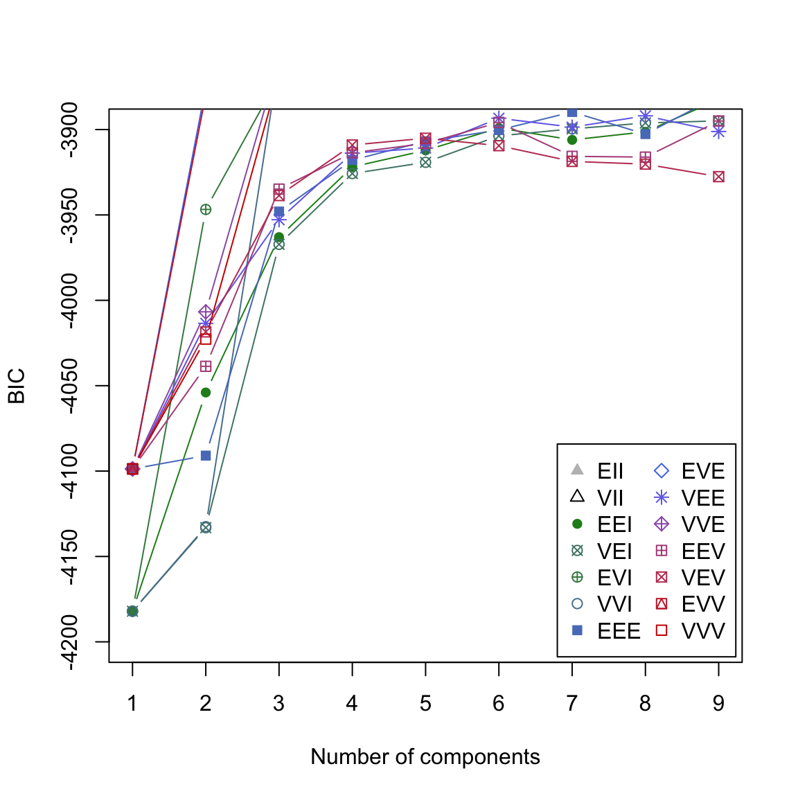

Use ?mclustModelNames to see descriptions for each of the model. This reveals that EEV only makes the simplifying assumption of equal volume between the different ellipsoids. This is also what you see in plot(gap2007_gm, what = 'classification').

plot(gap2007_gm, what = 'classification')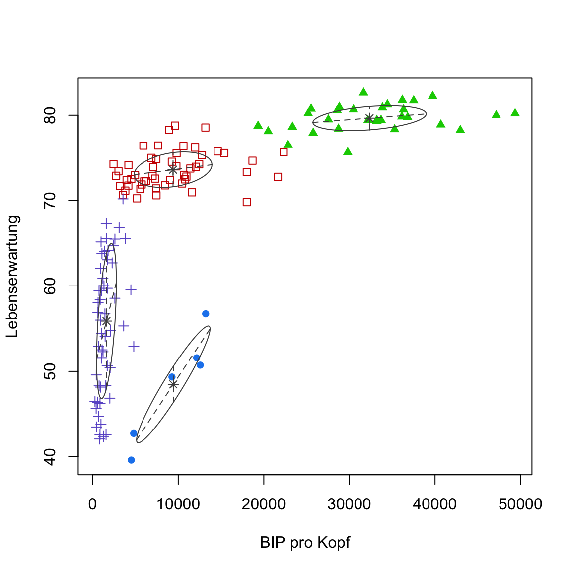

Now explore using the code below what happens if you tell the model to use a specific implementation of Gaussian mixtures. Replace the ‘XX’ in modelNames = 'XX' with one of the three letter codes denoting the different models. Then visualize the result. Begin with 'EEI'.

# Try different implementation
gap2007_gm <- Mclust(gap2007, modelNames = 'XX')
plot(gap2007_gm, what = 'classification')

# Try different implementation
gap2007_gm <- Mclust(gap2007, modelNames = 'EEI')
plot(gap2007_gm, what = 'classification')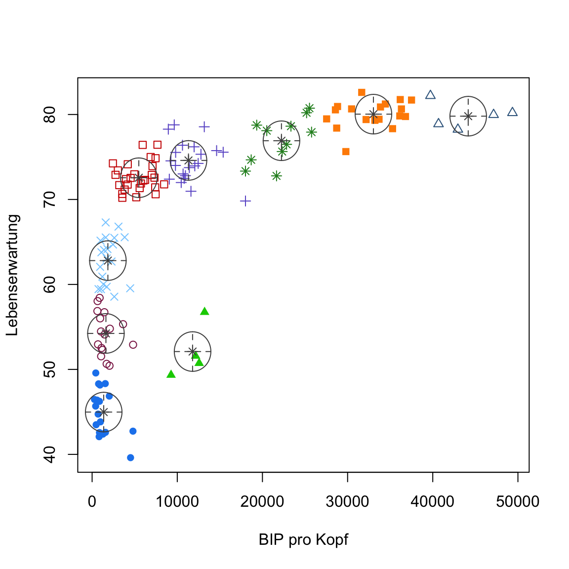

Y - Challenges: New data set

Use read_csv()to read in credit.csv as object credit.

# Read credit.csv
credit <- read_csv('1_Data/credit.csv')

Print the data set and familiarize yourself with its contents.
Use one or more of the clustering methods used above to identify clusters among credit card users. Have fun!

Examples

library(tidyverse) 
library(cstab)
library(dbscan)
library(mclust, mask.ok = F)

# Example data
data(mpg)

# Process data
mpg <- mpg %>% select_if(is.numeric)
mpg_stand <- mpg  %>% 
  scale %>%         # standardize/scale data
  as_tibble()

# k-means -----

# Identify clusters
mpg_km <- kmeans(mpg_stand, 
                 centers = 3)

# Show centroids
mpg_km$centers

# k-selection -----

# Sow within-variance 
km_development <- purrr::map(2:20, kmeans, x = mpg_stand)
withinvar <- purrr::map_dbl(km_development, 
                               `[[`, i = 'tot.withinss')

# Visualize withinvar
plot(withinvar)

# Gap & Slope statistics
k_est <- cDistance(as.matrix(mpg_stand), 
                   kseq = 2:20) 
k_est$k__Gap
k_est$k_Slope

# Cluster stability
k_est <- cStability(as.matrix(mpg_stand), 
                    kseq = 2:20) 
k_est$k_instab
  
# DBSCAN -----

# Identify clusters
mpg_dbscan <- dbscan(mpg_stand, eps = 1)

# Show centroids
mpg %>% 
  mutate(cl = mpg_dbscan$cluster) %>%
  group_by(cl) %>% 
  summarize_all(mean)

# Gaussian Mixtures -----

# Identify clusters
mpg_gm <- Mclust(mpg)

# Show centroids
mpg %>% 
  mutate(cl = mpg_gm$classification) %>%
  group_by(cl) %>% 
  summarize_all(mean)

# Visualize clusters
plot(mpg_gm, what = 'classification')

# Compare clusters -----

table(mpg_km$cluster, mpg_dbscan$cluster)
table(mpg_km$cluster, mpg_gm$classification)
table(mpg_dbscan$cluster, mpg_gm$classification)

Data sets

File	Rows	Columns
gap.csv	1692	6
credit.csv	8636	8

gap.csv

The gap data set is based on the Gapminder project and has been extracted from the R package gapminder.

Feature	Description
Land	Name of country
Kontinent	Name of continent
Jahr	year
Lebenserwartung	life expectancy in years
Population	Anzahl Population of country
BIP pro Kopf	GDP per capita

credit.csv

The credit data set is an excerpt of the publicly available Credit Card Dataset. The data set contains 8 features, that describe the behavior of 8636 credit card custmers.

Variable	Beschreibung
BALANCE	Available credit
BALANCE_FREQUENCY	Frequency of balance changes of (1 = frequent, 0 = infrequent)
PURCHASES	Sum of purchases
CREDITLIMIT	Limit of credit card
ONEOFFPURCHASES	Value of largest one-off purchase
MINIMUM_PAYMENTS	Minimal credit card payment
PRCFULLPAYMENT	Percent in-full credit card payments
TENURE	Duration of credit card account

Functions

Package

Paket	Installation
`tidyverse`	`install.packages("tidyverse")`
`cstab`	`install.packages("cstab")`
`dbscan`	`install.packages("dbscan")`
`mclust`	`install.packages("mclust")`

Functions

Clustering

Function	Package	Description
`kmeans()`	`stats`	Cluster data with k-means
`dbscan()`	`dbscan`	Cluster data with DBSCAN
`Mclust()`	`mclust`	Cluster data with Gaussian mixtures

k-selection

Function	Package	Description
`cDistance()`	`cstab`	Identify k with distance-based methods, e.g., gap statistic.
`cStability()`	`cstab`	Identify k with instability-based methods.

Resources

Documentation

A good Tutorial on k-means and hierarchical clustering.

Unsupervised learning

Machine learning with R The R Bootcamp

Overview

Tasks

A - Setup

B - Load the gap data set

C - k-means

D - k-selection

E - DBSCAN

F - Gaussian Mixtures

X - Challenges: Modellselection

Y - Challenges: New data set

Examples

Data sets

gap.csv

credit.csv

Functions

Package

Functions

Resources

Documentation

Machine learning with R
The R Bootcamp

B - Load the `gap` data set