Features
|
Machine Learning with R Basel R Bootcamp |

|

from from dilbert.com
Overview
By the end of this practical you will:
- Understand the importance of the curse of dimensionality.
- Know how to eliminate unwanted features.
- Explore and use feature importance.
- Use dimensionality reduction.
Tasks
A - Setup
Open your
BaselRBootcampR project. It should already have the folders1_Dataand2_Code. Make sure that the data file(s) listed in theDatasetssection are in your1_Datafolder.Open a new R script. At the top of the script, using comments, write your name and the date. Save it as a new file called
Features_practical.Rin the2_Codefolder.Using
library()load the set of packages for this practical listed in the packages section above.
# Load packages necessary for this script
library(tidyverse)
library(caret)- In the code below, we will load each of the data sets listed in the
Datasetsas new objects.
# Pima Indians diabetes
pima_diabetes <- read_csv(file = "1_Data/pima_diabetes.csv")

# (Non-) violent crime statistics
violent_crime    <- read_csv(file = "1_Data/violent_crime.csv")
nonviolent_crime <- read_csv(file = "1_Data/nonviolent_crime.csv")

# murders crime statistics
murders_crime <- read_csv(file = "1_Data/murders_crime.csv")
B - Pima Indians Diabetes
In this section, you will explore feature selection for the Pima Indians Diabetes data set. The Pima are a group of Native Americans living in Arizona. A genetic predisposition allowed this group to survive normally to a diet poor of carbohydrates for years. In the recent years, because of a sudden shift from traditional agricultural crops to processed foods, together with a decline in physical activity, made them develop the highest prevalence of type 2 diabetes. For this reason they have been subject of many studies.
- Take a look at the first few rows of the pima diabetes data frame by printing then to the console.
pima_diabetes# A tibble: 724 x 7
diabetes pregnant glucose pressure mass pedigree age
<chr> <dbl> <dbl> <dbl> <dbl> <dbl> <dbl>
1 pos 6 148 72 33.6 0.627 50
2 neg 1 85 66 26.6 0.351 31
3 pos 8 183 64 23.3 0.672 32
4 neg 1 89 66 28.1 0.167 21
5 pos 0 137 40 43.1 2.29 33
6 neg 5 116 74 25.6 0.201 30
7 pos 3 78 50 31 0.248 26
8 pos 2 197 70 30.5 0.158 53
9 neg 4 110 92 37.6 0.191 30
10 pos 10 168 74 38 0.537 34
# … with 714 more rows- Print the numbers of rows and columns of each data set using the
dim()function.
dim(pima_diabetes)[1] 724 7- Look at the names of the data frame with the
names()function.
names(pima_diabetes)[1] "diabetes" "pregnant" "glucose" "pressure" "mass" "pedigree"
[7] "age" - Open the data set in a new window using
View(). Do they look OK?
View(pima_diabetes)Splitting
- Before we begin, we need to make sure that we have a separate hold-out data set for later. Create
pima_trainandpima_testusing thecreateDataPartition()function. Setp = .15to select (only) 15% of cases for the training set. See code below. Also, store the variablediabetesfrom the test set as a factor, which will be the criterion.
# split index
train_index <- createDataPartition(XX$XX, p = .15, list = FALSE)

# train and test sets
pima_train <- XX %>% slice(train_index)
pima_test  <- XX %>% slice(-train_index)

# test criterion
criterion <- as.factor(pima_test$XX)
# split index
train_index <- createDataPartition(pima_diabetes$diabetes, p = .15, list = FALSE)
# train and test sets
pima_train <- pima_diabetes %>% slice(train_index)
pima_test <- pima_diabetes %>% slice(-train_index)
# test criterion
criterion <- as.factor(pima_test$diabetes)Remove unwanted features
OK, with the training set, let’s get to work and remove some features.
- First split the training data into a data frame holding the predictors and a vector holding the criterion using the template below.
# Select predictors
pima_train_pred <- pima_train %>% select(-XX)

# Select criterion
pima_train_crit <- pima_train %>% pull(XX)
# Select predictors
pima_train_pred <- pima_train %>% select(-diabetes)
# Select criterion
pima_train_crit <- pima_train %>% pull(diabetes)- Although, this data set is rather small and well curated, test using the template below whether there are any excessively correlated features using
cor()andfindCorrelation(). Are there any?
# determine correlation matrix
corr_matrix <- cor(XX_pred)

# find excessively correlated variables
findCorrelation(corr_matrix)
# determine correlation matrix
corr_matrix <- cor(pima_train_pred)
# find excessively correlated variables
findCorrelation(corr_matrix)integer(0)- Now, test if there are any near-zero variance features using the
nearZeroVarfunction. Any of those?
# find near zero variance predictors
nearZeroVar(XX_pred)
# find near zero variance predictors
nearZeroVar(pima_train_pred)integer(0)Feature importance
As we identified no problems with the features in our data set, we have retained all of them. In this section, you will carry out feature selection on grounds of feature importance. To do this, we first need to fit a model on the basis of which we can determine the importance of features. How about using a simple logistic regression aka method = "glm"?
- Fit a
glmmodel to the training data.
# fit regression
pima_glm <- train(diabetes ~ .,
                data = XX,
                method = XX
                )
# fit regression
pima_glm <- train(diabetes ~ .,
data = pima_train,
method = "glm")- Evaluate feature importance using
varImp(). The function will show importance on a scale from 0 (least important feature) to 100 (most important feature). You can setscale = TRUEto see absolute importance measures scaled as t-values.
# determine variable importance
varimp_glm <- varImp(XX)

# print variable importance
varimp_glm

# print variable importance
plot(varimp_glm)
# determine variable importance
varimp_glm <- varImp(pima_glm)
# print variable importance
varimp_glmglm variable importance
Overall
glucose 100.00
mass 76.21
age 52.67
pregnant 10.72
pedigree 2.02
pressure 0.00# print variable importance
plot(varimp_glm)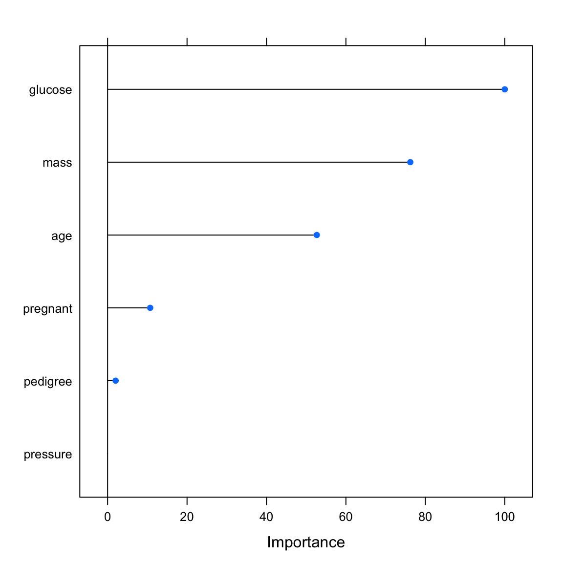
Model comparison
Now, let’s create a second model using the best features and compare performances.
- Fit the glm a second time, this time using only the four best features and store the result in a different fit object.
# fit glm with best four features
pima_glm4 <- train(diabetes ~ XX + YY + ZZ + AA,
                data = XX,
                method = XX)
# fit glm with best four features
pima_glm4 <- train(diabetes ~ glucose + mass + pregnant + pedigree,
data = pima_train,
method = "glm")- Using the fit of the model containing all features versus the one using the best four, predict the criterion and evaluate the prediction using
confusionMatrix(). Which model model is better?
# determine predictions for test data
pima_glm_pred <- predict(XX, newdata = XX)
pima_glm4_pred <- predict(XX, newdata = XX)

# evaluate the results
confusionMatrix(XX, reference = XX)
confusionMatrix(XX, reference = XX)
# determine predictions for test data
pima_glm_pred <- predict(pima_glm, newdata = pima_test)
pima_glm4_pred <- predict(pima_glm4, newdata = pima_test)
# evaluate the results
confusionMatrix(pima_glm_pred, criterion)Confusion Matrix and Statistics
Reference
Prediction neg pos
neg 344 89
pos 59 122
Accuracy : 0.759
95% CI : (0.723, 0.792)
No Information Rate : 0.656
P-Value [Acc > NIR] : 2.34e-08
Kappa : 0.447
Mcnemar's Test P-Value : 0.0171
Sensitivity : 0.854
Specificity : 0.578
Pos Pred Value : 0.794
Neg Pred Value : 0.674
Prevalence : 0.656
Detection Rate : 0.560
Detection Prevalence : 0.705
Balanced Accuracy : 0.716
'Positive' Class : neg
confusionMatrix(pima_glm4_pred, criterion)Confusion Matrix and Statistics
Reference
Prediction neg pos
neg 353 96
pos 50 115
Accuracy : 0.762
95% CI : (0.727, 0.795)
No Information Rate : 0.656
P-Value [Acc > NIR] : 8.3e-09
Kappa : 0.444
Mcnemar's Test P-Value : 0.000196
Sensitivity : 0.876
Specificity : 0.545
Pos Pred Value : 0.786
Neg Pred Value : 0.697
Prevalence : 0.656
Detection Rate : 0.575
Detection Prevalence : 0.731
Balanced Accuracy : 0.710
'Positive' Class : neg
You might have observed that the model with two fewer features is actually slightly better than the full model (if this is not the case, keep in mind that the partitioning of the dataset was done randomly, i.e., if you do it a second time, your results may slightly change). Why do you think this is the case?
Play around: Up the proportion dedicated to training or use a different model, e.g.,
random forest, and see whether things change.
C - Murders
In this section, you will explore feature selection using a different data set. The data combines socio-economic data from the US ’90 Census, data from Law Enforcement Management and Admin Stats survey, and crime data from the FB. The gaol of this section is to use various socio-demographic variables to predict whether murders have been committed (murders), the criterion of this exercise.
- Take a look at the first few rows of the
murders_crimedata frame by printing them to the console.
murders_crime# A tibble: 1,823 x 102
murders population householdsize racepctblack racePctWhite racePctAsian
<chr> <dbl> <dbl> <dbl> <dbl> <dbl>
1 yes 27591 2.63 0.17 94.8 1.6
2 yes 36830 2.6 42.4 53.7 0.54
3 yes 23928 2.6 11.0 81.3 1.78
4 no 15675 2.59 4.08 84.1 0.54
5 yes 96086 3.19 8.54 59.8 17.2
6 no 48622 2.44 3.14 95.5 0.77
7 no 10444 3.02 0.41 98.9 0.39
8 yes 222103 2.49 11.4 82.4 3.77
9 no 15535 2.35 14.9 84.6 0.32
10 yes 24664 2.73 13.7 85.0 0.53
# … with 1,813 more rows, and 96 more variables: racePctHisp <dbl>,
# agePct12t21 <dbl>, agePct12t29 <dbl>, agePct16t24 <dbl>,
# agePct65up <dbl>, numbUrban <dbl>, pctUrban <dbl>, medIncome <dbl>,
# pctWWage <dbl>, pctWFarmSelf <dbl>, pctWInvInc <dbl>,
# pctWSocSec <dbl>, pctWPubAsst <dbl>, pctWRetire <dbl>,
# medFamInc <dbl>, perCapInc <dbl>, whitePerCap <dbl>,
# blackPerCap <dbl>, indianPerCap <dbl>, AsianPerCap <dbl>,
# HispPerCap <dbl>, NumUnderPov <dbl>, PctPopUnderPov <dbl>,
# PctLess9thGrade <dbl>, PctNotHSGrad <dbl>, PctBSorMore <dbl>,
# PctUnemployed <dbl>, PctEmploy <dbl>, PctEmplManu <dbl>,
# PctEmplProfServ <dbl>, PctOccupManu <dbl>, PctOccupMgmtProf <dbl>,
# MalePctDivorce <dbl>, MalePctNevMarr <dbl>, FemalePctDiv <dbl>,
# TotalPctDiv <dbl>, PersPerFam <dbl>, PctFam2Par <dbl>,
# PctKids2Par <dbl>, PctYoungKids2Par <dbl>, PctTeen2Par <dbl>,
# PctWorkMomYoungKids <dbl>, PctWorkMom <dbl>,
# NumKidsBornNeverMar <dbl>, PctKidsBornNeverMar <dbl>, NumImmig <dbl>,
# PctImmigRecent <dbl>, PctImmigRec5 <dbl>, PctImmigRec8 <dbl>,
# PctImmigRec10 <dbl>, PctRecentImmig <dbl>, PctRecImmig5 <dbl>,
# PctRecImmig8 <dbl>, PctRecImmig10 <dbl>, PctSpeakEnglOnly <dbl>,
# PctNotSpeakEnglWell <dbl>, PctLargHouseFam <dbl>,
# PctLargHouseOccup <dbl>, PersPerOccupHous <dbl>,
# PersPerOwnOccHous <dbl>, PersPerRentOccHous <dbl>,
# PctPersOwnOccup <dbl>, PctPersDenseHous <dbl>, PctHousLess3BR <dbl>,
# MedNumBR <dbl>, HousVacant <dbl>, PctHousOccup <dbl>,
# PctHousOwnOcc <dbl>, PctVacantBoarded <dbl>, PctVacMore6Mos <dbl>,
# MedYrHousBuilt <dbl>, PctHousNoPhone <dbl>, PctWOFullPlumb <dbl>,
# OwnOccLowQuart <dbl>, OwnOccMedVal <dbl>, OwnOccHiQuart <dbl>,
# OwnOccQrange <dbl>, RentLowQ <dbl>, RentMedian <dbl>, RentHighQ <dbl>,
# RentQrange <dbl>, MedRent <dbl>, MedRentPctHousInc <dbl>,
# MedOwnCostPctInc <dbl>, MedOwnCostPctIncNoMtg <dbl>,
# NumInShelters <dbl>, NumStreet <dbl>, PctForeignBorn <dbl>,
# PctBornSameState <dbl>, PctSameHouse85 <dbl>, PctSameCity85 <dbl>,
# PctSameState85 <dbl>, LandArea <dbl>, PopDens <dbl>,
# PctUsePubTrans <dbl>, LemasPctOfficDrugUn <dbl>- Print the numbers of rows and columns of each data set using the
dim()function.
dim(murders_crime)[1] 1823 102- Look at the names of the data frame with the
names()function.
names(murders_crime) [1] "murders" "population"
[3] "householdsize" "racepctblack"
[5] "racePctWhite" "racePctAsian"
[7] "racePctHisp" "agePct12t21"
[9] "agePct12t29" "agePct16t24"
[11] "agePct65up" "numbUrban"
[13] "pctUrban" "medIncome"
[15] "pctWWage" "pctWFarmSelf"
[17] "pctWInvInc" "pctWSocSec"
[19] "pctWPubAsst" "pctWRetire"
[21] "medFamInc" "perCapInc"
[23] "whitePerCap" "blackPerCap"
[25] "indianPerCap" "AsianPerCap"
[27] "HispPerCap" "NumUnderPov"
[29] "PctPopUnderPov" "PctLess9thGrade"
[31] "PctNotHSGrad" "PctBSorMore"
[33] "PctUnemployed" "PctEmploy"
[35] "PctEmplManu" "PctEmplProfServ"
[37] "PctOccupManu" "PctOccupMgmtProf"
[39] "MalePctDivorce" "MalePctNevMarr"
[41] "FemalePctDiv" "TotalPctDiv"
[43] "PersPerFam" "PctFam2Par"
[45] "PctKids2Par" "PctYoungKids2Par"
[47] "PctTeen2Par" "PctWorkMomYoungKids"
[49] "PctWorkMom" "NumKidsBornNeverMar"
[51] "PctKidsBornNeverMar" "NumImmig"
[53] "PctImmigRecent" "PctImmigRec5"
[55] "PctImmigRec8" "PctImmigRec10"
[57] "PctRecentImmig" "PctRecImmig5"
[59] "PctRecImmig8" "PctRecImmig10"
[61] "PctSpeakEnglOnly" "PctNotSpeakEnglWell"
[63] "PctLargHouseFam" "PctLargHouseOccup"
[65] "PersPerOccupHous" "PersPerOwnOccHous"
[67] "PersPerRentOccHous" "PctPersOwnOccup"
[69] "PctPersDenseHous" "PctHousLess3BR"
[71] "MedNumBR" "HousVacant"
[73] "PctHousOccup" "PctHousOwnOcc"
[75] "PctVacantBoarded" "PctVacMore6Mos"
[77] "MedYrHousBuilt" "PctHousNoPhone"
[79] "PctWOFullPlumb" "OwnOccLowQuart"
[81] "OwnOccMedVal" "OwnOccHiQuart"
[83] "OwnOccQrange" "RentLowQ"
[85] "RentMedian" "RentHighQ"
[87] "RentQrange" "MedRent"
[89] "MedRentPctHousInc" "MedOwnCostPctInc"
[91] "MedOwnCostPctIncNoMtg" "NumInShelters"
[93] "NumStreet" "PctForeignBorn"
[95] "PctBornSameState" "PctSameHouse85"
[97] "PctSameCity85" "PctSameState85"
[99] "LandArea" "PopDens"
[101] "PctUsePubTrans" "LemasPctOfficDrugUn" - Open the data set in a new window using
View(). Do they look OK?
View(murders_crime)Splitting
- Again, let us first create a hold-out data set for later. Create
murders_trainandmurders_testusingcreateDataPartition()with (only) 25% of cases going into the training set. Also store the variablemurdersfrom the test, i.e., the criterion, and turn into a factor usingas.factor().
# split index
train_index <- createDataPartition(murders_crime$murders, p = .25, list = FALSE)

# train and test sets
murders_train <- murders_crime %>% slice(train_index)
murders_test  <- murders_crime %>% slice(-train_index)

# test criterion
criterion <- as.factor(murders_test$murders)
Remove unwanted features
Before we start modeling, let us get to work and remove some features from the training set.
- To this end, first split the training data into a data frame holding the predictors and the criterion in the same way you have done this above.
# Select predictors
murders_train_pred <- murders_train %>% select(-murders)

# Select criterion
murders_train_crit <- murders_train %>% select(murders) %>% pull()- Test if there are any excessively correlated features using
cor()andfindCorrelation(). Are there any this time?
# determine correlation matrix
corr_matrix <- cor(murders_train_pred)

# find excessively correlated variables
findCorrelation(corr_matrix)
[1] 11 17 27 30 41 44 51 53 54 55 57 58 59 61 64 71 84 85 87 7 8 13 20
[24] 21 31 38 43 1 62 67 79 80 81- Using the code below, remove the excessively correlated features from the training predictor set.
# remove features
murders_train_pred <- murders_train_pred %>% select(- XX)
# remove features
murders_train_pred <- murders_train_pred %>%
select(-findCorrelation(corr_matrix))- Test if there are any near-zero variance features. Any of those this time?
# find near zero variance predictors
nearZeroVar(murders_train_pred)integer(0)- You should have found that there were plenty of excessively correlated features but no near-zero variance features. Provided that you excluded some of the former, bind the reduced predictor set back together with the criterion into a new, clean version of the training set. See template below.
# clean training set
murders_train_clean <- murders_train_pred %>%
  add_column(murders = XX)
# combine clean predictor set with criterion
murders_train_clean <- murders_train_pred %>%
add_column(murders = murders_train_crit)Model comparison
- Let us find out whether excluding some of the highly correlated features matters. Fit a
glmtwice, once using the original training set and once using the clean training set, and store the fits in separate objects. See template below.
# fit glm
murders_glm <- train(murders ~ .,
                     data = XX,
                     method = "glm")

# fit glm with clean data
murders_glm_clean <- train(murders ~ .,
                           data = XX,
                           method = "glm")
# fit glm
murders_glm <- train(murders ~ .,
data = murders_train,
method = "glm")
# fit glm with clean data
murders_glm_clean <- train(murders ~ .,
data = murders_train_clean,
method = "glm")- You probably have noticed warning messages. They concern the very fact that the features in both data sets, but especially the non-clean set, are still too highly correlated. Go ahead and evaluate the performance on the hold-out set. Which set of features predicts better?
# determine predictions for test data
murders_pred <- predict(murders_glm, newdata = murders_test)
murders_clean_pred <- predict(murders_glm_clean, newdata = murders_test)

# evaluate the results
confusionMatrix(murders_pred, criterion)
Confusion Matrix and Statistics
Reference
Prediction no yes
no 446 192
yes 184 545
Accuracy : 0.725
95% CI : (0.7, 0.748)
No Information Rate : 0.539
P-Value [Acc > NIR] : <2e-16
Kappa : 0.447
Mcnemar's Test P-Value : 0.718
Sensitivity : 0.708
Specificity : 0.739
Pos Pred Value : 0.699
Neg Pred Value : 0.748
Prevalence : 0.461
Detection Rate : 0.326
Detection Prevalence : 0.467
Balanced Accuracy : 0.724
'Positive' Class : no
confusionMatrix(murders_clean_pred, criterion)Confusion Matrix and Statistics
Reference
Prediction no yes
no 471 199
yes 159 538
Accuracy : 0.738
95% CI : (0.714, 0.761)
No Information Rate : 0.539
P-Value [Acc > NIR] : <2e-16
Kappa : 0.475
Mcnemar's Test P-Value : 0.0393
Sensitivity : 0.748
Specificity : 0.730
Pos Pred Value : 0.703
Neg Pred Value : 0.772
Prevalence : 0.461
Detection Rate : 0.345
Detection Prevalence : 0.490
Balanced Accuracy : 0.739
'Positive' Class : no
Data compression with PCA
- Given the high features correlations, it is sensible to compress the data using
principal component analysis(PCA). Create a third fit object using the original, full training set using againmethod = glmand in additionpreProcess = c('pca')andtrControl = trainControl(preProcOptions = list(thresh = 0.8))in the training function. These additional settings instruct R to extract new features from the data using PCA and to retain only as many features as are needed to capture 80% of the original variance.
# fit glm with preprocessed features
murders_glm_pca = train(murders ~ .,
                        data = murders_train,
                        method = "glm",
                        preProcess = c("pca"),
trControl = trainControl(preProcOptions = list(thresh = 0.8)))- Compare the prediction performance to the previous two models.
# determine predictions for test data
murders_pca <- predict(murders_glm_pca, newdata = murders_test)

# evaluate the results
confusionMatrix(murders_pca, criterion)
Confusion Matrix and Statistics
Reference
Prediction no yes
no 490 196
yes 140 541
Accuracy : 0.754
95% CI : (0.73, 0.777)
No Information Rate : 0.539
P-Value [Acc > NIR] : <2e-16
Kappa : 0.509
Mcnemar's Test P-Value : 0.0027
Sensitivity : 0.778
Specificity : 0.734
Pos Pred Value : 0.714
Neg Pred Value : 0.794
Prevalence : 0.461
Detection Rate : 0.358
Detection Prevalence : 0.502
Balanced Accuracy : 0.756
'Positive' Class : no
- Play around: Alter the amount of variance explained by the
PCA(usingthresh), increase the proportion dedicated to training, use a different model, e.g.,random forest, and see whether things change.
Feature importance
- Now let’s find out, which features are most important for predicting murders. Using
varImp(), evaluate the feature importance for each of the three models used in the previous section.
# determine variable importance
varimp_glm <- varImp(murders_glm)
varimp_glm_clean <- varImp(murders_glm_clean)
varimp_glm_pca <- varImp(murders_glm_pca)

# print variable importance
varimp_glm
glm variable importance
only 20 most important variables shown (out of 99)
Overall
PctForeignBorn 100.0
PctNotSpeakEnglWell 98.2
pctWRetire 97.8
PersPerFam 85.7
PctKidsBornNeverMar 82.0
racepctblack 81.1
PctFam2Par 81.1
PctHousNoPhone 75.6
NumUnderPov 74.3
racePctAsian 73.6
NumStreet 71.7
agePct12t21 69.4
PctKids2Par 65.7
PctBornSameState 63.2
population 58.8
PctOccupManu 57.9
pctWSocSec 57.8
PctEmplManu 56.2
MedRentPctHousInc 52.7
blackPerCap 50.1varimp_glm_cleanglm variable importance
only 20 most important variables shown (out of 68)
Overall
NumKidsBornNeverMar 100.0
PctKidsBornNeverMar 79.5
PctEmplManu 61.4
PctHousOccup 56.2
MedRentPctHousInc 54.1
PctOccupManu 48.8
pctWRetire 48.2
PctHousNoPhone 46.7
PctUsePubTrans 46.3
PctBornSameState 45.4
racepctblack 45.3
PersPerFam 42.5
PctForeignBorn 39.9
OwnOccQrange 39.1
pctWPubAsst 38.4
PctRecentImmig 35.4
MedOwnCostPctInc 34.8
PctOccupMgmtProf 34.7
FemalePctDiv 34.5
racePctAsian 34.1varimp_glm_pcaglm variable importance
Overall
PC1 100.00
PC2 94.19
PC4 80.80
PC3 77.90
PC5 74.74
PC11 60.11
PC8 48.74
PC6 35.34
PC7 32.85
PC9 9.67
PC10 0.00# print variable importance
plot(varimp_glm)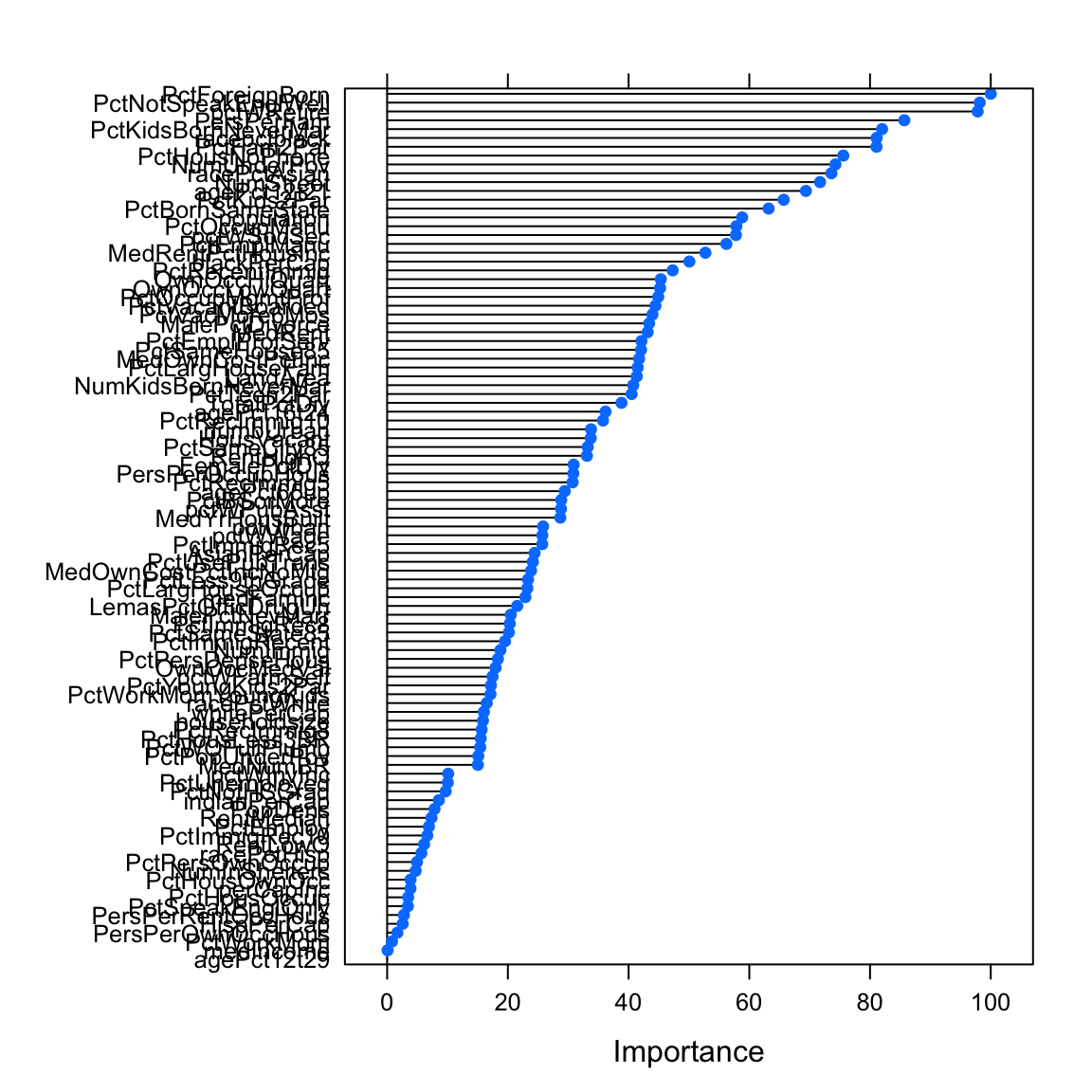
plot(varimp_glm_clean)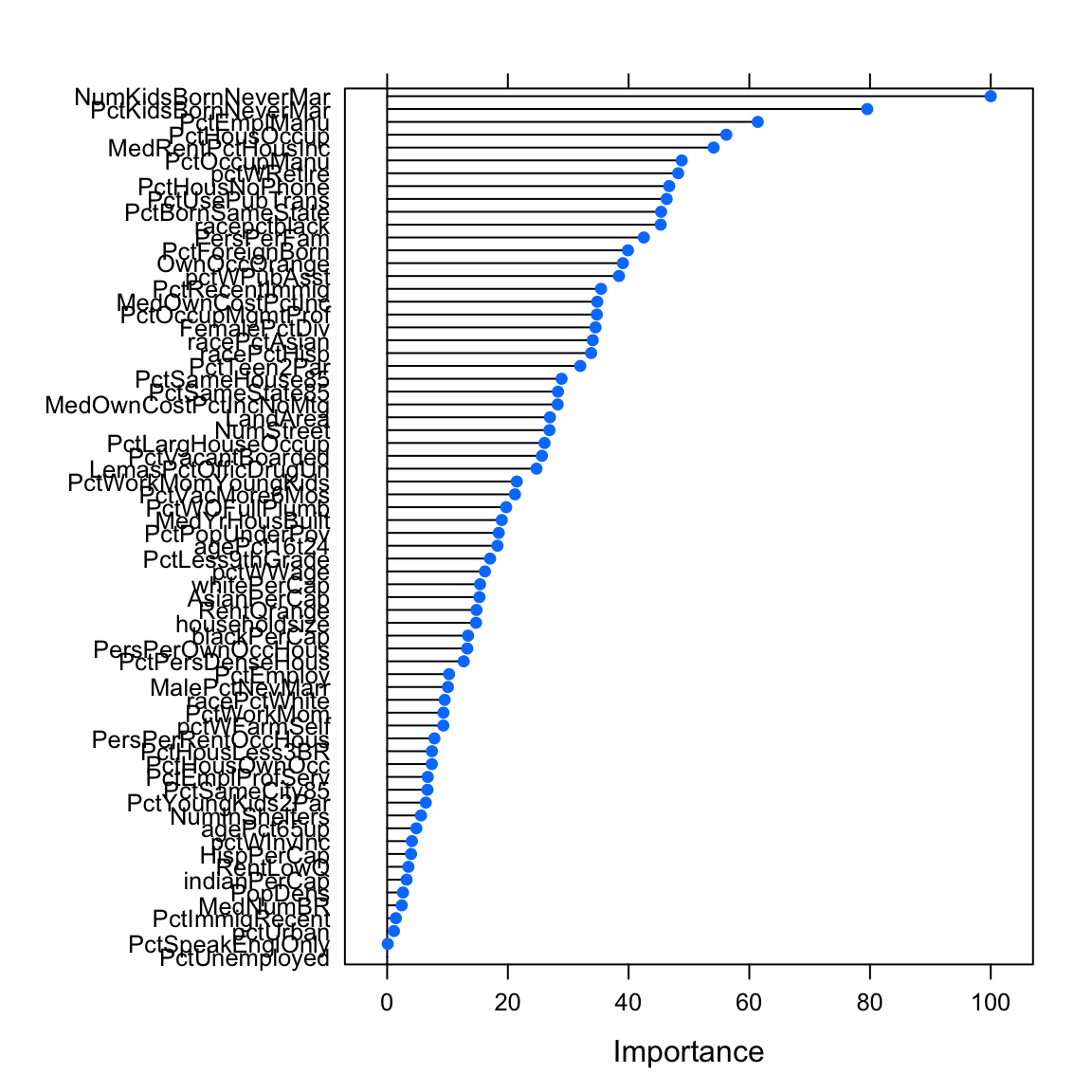
plot(varimp_glm_pca)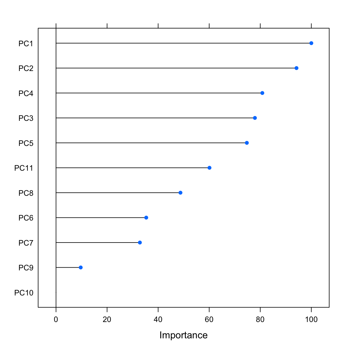
- Now that you know which features were most important, do you think you can come up with a set of features that reliably outperforms thew predictions based on the pca-generated feature set? Try it out!
Z - Violent & Non-violent Crime Data
Analyze the violent and non-violent crime data sets predicting either the number of violent crimes per 100k inhabitants (
ViolentCrimesPerPop) or the number of non-violent crimes per 100k inhabitants (nonViolPerPop). Both criteria are numeric, implying that this is not classification problem, but one of regression. Other than that, the features in the data set are identical to the previous analyses. How well can you predict violent or non-violent crimes?Another approach to feature selection, beyond selection by hand or PCA, is to have the computer try to automically select subsets of features that lead to the best possible cross-validation performance. One such process is called recursive feature elimination. Try it out using
caret’srfe()function. See code below.
# split index
train_index <- createDataPartition(violent_crime$ViolentCrimesPerPop,
                                   p = .8,
                                   list = FALSE)

# train and test sets
violent_train <- violent_crime %>% slice(train_index)
violent_test  <- violent_crime %>% slice(-train_index)

# remove extreme correlations (OPTIONAL)
predictors <- violent_train %>% select(-ViolentCrimesPerPop)
predictors <- predictors %>% select(-findCorrelation(cor(predictors)))
violent_train_clean <- predictors %>%
  add_column(ViolentCrimesPerPop = violent_train$ViolentCrimesPerPop)

# Feature elimination settings
ctrl_rfe <- rfeControl(functions = lmFuncs,  # linear model
                          method = "cv",
                          verbose = FALSE,
                          rerank = FALSE)

# Run feature elimination
profile <- rfe(x = violent_train %>% select(-ViolentCrimesPerPop),
               y = violent_train$ViolentCrimesPerPop,
               sizes = 1:(ncol(violent_train_clean)-1), # Features set sizes
               rfeControl = ctrl_rfe)

# inspect cross-validation as a function of performance
plot(profile)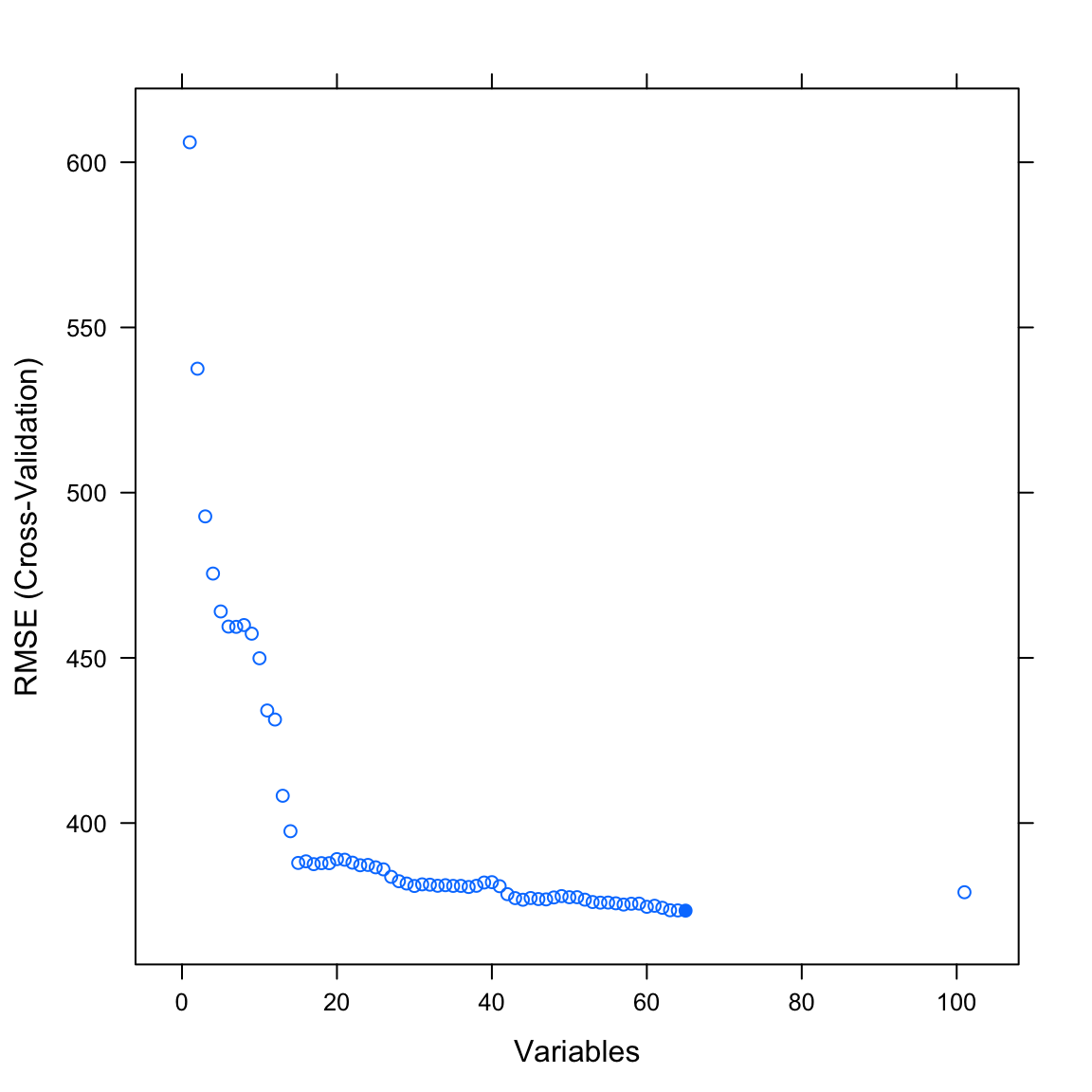
Examples
# Step 0: Load packages-----------

library(tidyverse)    # Load tidyverse for dplyr and tidyr
library(tibble)       # For advanced tibble functions
library(caret)        # For ML mastery

# Step 1: Load, prepare, and explore data ----------------------

# read data
data <- read_csv("1_Data/mpg_num.csv")

# Convert all characters to factors
data <- data %>%
  mutate_if(is.character, factor)

# Explore training data
data        # Print the dataset
dim(data)   # Print dimensions
names(data) # Print the names

# Step 2: Create training and test sets -------------

# Create train index
train_index <- createDataPartition(criterion,
                                   p = .8,
                                   list = FALSE)

# Create training and test sets
data_train <- data %>% slice(train_index)
data_test <- data %>% slice(-train_index)

# split predictors and criterion
criterion_train <- data_train %>% select(hwy) %>% pull()
predictors_train <- data_train %>% select(-hwy)
criterion_test <- data_test %>% select(hwy) %>% pull()
predictors_test <- data_test %>% select(-hwy)

# Step 3: Clean data -------------

# Test for excessively correlated features
corr_matrix <- cor(predictors_train)
corr_features <- findCorrelation(corr_matrix)

# Remove excessively correlated features
predictors_train <- predictors_train %>% select(-corr_features)

# Test for near zero variance features
zerovar_features <- nearZeroVar(predictors_train)

# Remove near zero variance features
predictors_train <- predictors_train %>% select(-zerovar_features)

# recombine data
data_train <- predictors_train %>% add_column(hwy = criterion_train)

# Step 4: Define training control parameters -------------

# Train using cross-validation
ctrl_cv <- trainControl(method = "cv")

# Step 5: Fit models -------------

# Fit glm vanilla flavor
hwy_glm <- train(form = hwy ~ .,
                 data = data_train,
                 method = "glm",
                 trControl = ctrl_cv)

# Fit with pca transformation
hwy_glm_pca <- train(form = hwy ~ .,
                     data = data_train,
                     method = "glm",
                     trControl = ctrl_cv,
                     preProcess = c('pca'))

# Fit scaling and centering
hwy_glm_sca <- train(form = hwy ~ .,
                     data = data_train,
                     method = "glm",
                     trControl = ctrl_cv,
                     preProcess = c('scale', 'center'))

# Get fits
glm_fit     <- predict(hwy_glm)
glm_pca_fit <- predict(hwy_glm_pca)
glm_sca_fit <- predict(hwy_glm_sca)

# Step 6: Evaluate variable importance -------------

# Run varImp()
imp_glm     <- varImp(hwy_glm)
imp_glm_pca <- varImp(hwy_glm_pca)
imp_glm_sca <- varImp(hwy_glm_sca)

# Plot variable importance
plot(imp_glm)
plot(imp_glm_pca)
plot(imp_glm_sca)

# Step 7: Select variables -------------

# Select by hand in formula
hwy_glm_sel <- train(form = hwy ~ cty,
                     data = data_train,
                     method = "glm",
                     trControl = ctrl_cv)

# Select by reducing pca criterion ---

# Reduce criterion to 50% variance epxlained
ctrl_cv_pca <- trainControl(method = "cv",
                            preProcOptions = list(thresh = 0.50))

# Refit model with update
hwy_glm_sel <- train(form = hwy ~ .,
                     data = data_train,
                     method = "glm",
                     trControl = ctrl_cv_pca,
                     preProcess = c('pca'))

# Step 8: Recursive feature elimination -------------

# Feature elimination settings
ctrl_rfe <- rfeControl(functions = lmFuncs,  # linear model
                       method = "cv",
                       verbose = FALSE)

# Run feature elimination
profile <- rfe(x = predictors_train,
               y = criterion_train,
               sizes = c(1, 2, 3),     # Features set sizes should be considered
               rfeControl = ctrl_rfe)

# plot result
trellis.par.set(caretTheme())
plot(profile, type = c("g", "o"))

# Step 9: Evaluate models -------------

# you know how...
Datasets
| File | Rows | Columns |
|---|---|---|
| pima_diabetes | 724 | 7 |
| murders_crime | 1000 | 102 |
| violent_crime | 1000 | 102 |
| nonviolent_crime | 1000 | 102 |
The
pima_diabetesis a subset of thePimaIndiansDiabetes2data set in themlbenchpackage. It contains medical and demographic data of Pima Indians.The
murders_crime,violent_crime, andnon_violent_crimedata are subsets of the Communities and Crime Unnormalized Data Set data set from the UCI Machine Learning Repository. To see column descriptions, visit this site: Communities and Crime Unnormalized Data Set. Due to the large number of variables (102), we do not include the full tables below.
Variable description of pima_diabetes
| Name | Description |
|---|---|
pregnant |
Number of times pregnant. |
glucose |
Plasma glucose concentration (glucose tolerance test). |
pressure |
Diastolic blood pressure (mm Hg). |
triceps |
Triceps skin fold thickness (mm). |
insulin |
2-Hour serum insulin (mu U/ml). |
mass |
Body mass index (weight in kg/(height in m)^2). |
pedigree |
Diabetes pedigree function. |
age |
Age (years). |
diabetes |
Class variable (test for diabetes). |
Functions
Packages
| Package | Installation |
|---|---|
tidyverse |
install.packages("tidyverse") |
tibble |
install.packages("tibble") |
caret |
install.packages("caret") |
Functions
| Function | Package | Description |
|---|---|---|
trainControl() |
caret |
Define modelling control parameters |
train() |
caret |
Train a model |
predict(object, newdata) |
stats |
Predict the criterion values of newdata based on object |
postResample() |
caret |
Calculate aggregate model performance in regression tasks |
confusionMatrix() |
caret |
Calculate aggregate model performance in classification tasks |
varImp() |
caret |
Determine the model-specific importance of features |
findCorrelation(), nearZeroVar() |
caret |
Identify highly correlated and low variance features. |
rfe(), rfeControl() |
caret |
Run and control recursive feature selection. |
Resources
Cheatsheet
from github.com/rstudio