Optimization
|
Machine Learning with R Basel R Bootcamp |

|
from xkcd.com
Overview
By the end of this practical you will know how to:
- Use cross-validation to select optimal model tuning parameters for decision trees and random forests.
- Compare ‘standard’ regression with lasso and ridge penalised regression.
- Use cross-validation to estimate future test accuracy.
Tasks
Baseball player salaries
In this practical, we will predict the Salary of baseball players from the hitters_train and hitters_test datasets.
A - Setup
Open your
BaselRBootcampR project. It should already have the folders1_Dataand2_Code. Make sure that the data file(s) listed in theDatasetssection are in your1_DatafolderOpen a new R script. At the top of the script, using comments, write your name and the date. Save it as a new file called
Optimization_practical.Rin the2_Codefolder.Using
library()load the set of packages for this practical listed in the packages section above.
# Load packages necessary for this script
library(tidyverse)
library(caret)
library(party)
library(partykit)- Run the code below to load each of the datasets listed in the
Datasetssection as new objects.
# hitters data
hitters_train <- read_csv(file = "1_Data/hitters_train.csv")
hitters_test <- read_csv(file = "1_Data/hitters_test.csv")- Take a look at the first few rows of each dataframe by printing them to the console.
# Print dataframes to the console
hitters_train
hitters_test- Print the numbers of rows and columns of each dataset using the
dim()function.
# Print numbers of rows and columns
dim(XXX)
dim(XXX)dim(hitters_train)[1] 50 20dim(hitters_test)[1] 213 20- Look at the names of the dataframes with the
names()function.
# Print the names of each dataframe
names(XXX)
names(XXX)
names(hitters_train) [1] "Salary" "AtBat" "Hits" "HmRun" "Runs"
[6] "RBI" "Walks" "Years" "CAtBat" "CHits"
[11] "CHmRun" "CRuns" "CRBI" "CWalks" "League"
[16] "Division" "PutOuts" "Assists" "Errors" "NewLeague"names(hitters_test) [1] "Salary" "AtBat" "Hits" "HmRun" "Runs"
[6] "RBI" "Walks" "Years" "CAtBat" "CHits"
[11] "CHmRun" "CRuns" "CRBI" "CWalks" "League"
[16] "Division" "PutOuts" "Assists" "Errors" "NewLeague"- Open each dataset in a new window using
View(). Do they look ok?
# Open each dataset in a window.
View(XXX)
View(XXX)- As always, we need to convert all character columns to factors before we start. Do this by running the following code.
# Convert all character columns to factor
hitters_train <- hitters_train %>%
          mutate_if(is.character, factor)

hitters_test <- hitters_test %>%
          mutate_if(is.character, factor)
B - Setup trainControl
- Set up your training by specifying
ctrl_cvas 10-fold cross-validation. Specifically,…
- set
method = "cv"to specify cross validation. - set
number = 10to specify 10 folds.
# Use 10-fold cross validation
ctrl_cv <- trainControl(method = "XX",
                        number = XX)
# Use 10-fold cross validation
ctrl_cv <- trainControl(method = "cv",
number = 10) C - Regression (standard)
- Fit a (standard) regression model predicting
Salaryas a function of all features. Specifically,…
- set the formula to
Salary ~ .. - set the data to
hitters_train. - set the method to
"glm"for regular regression. - set the train control argument to
ctrl_cv.
# Normal Regression --------------------------
salary_glm <- train(form = XX ~ .,
data = XX,
method = "XX",
trControl = XX)# Normal Regression --------------------------
salary_glm <- train(form = Salary ~ .,
data = hitters_train,
method = "glm",
trControl = ctrl_cv)- Print your
salary_glm. What do you see?
salary_glmGeneralized Linear Model
50 samples
19 predictors
No pre-processing
Resampling: Cross-Validated (10 fold)
Summary of sample sizes: 43, 45, 45, 46, 45, 46, ...
Resampling results:
RMSE Rsquared MAE
575 0.377 490- Try plotting your
salary_glmobject. What happens? What does this error mean?
# I get the following error:
# Error in plot.train(salary_glm) :
# There are no tuning parameters for this model.
# The problem is that method = "glm" has no tuning parameters so there is nothing to plot!- Print your final model object with
salary_glm$finalModel.
# Print final regression model
salary_glm$finalModel
Call: NULL
Coefficients:
(Intercept) AtBat Hits HmRun Runs
664.0169 -1.8086 12.7263 14.0206 -10.7594
RBI Walks Years CAtBat CHits
-5.1859 -8.6702 -62.3666 0.4883 -4.9553
CHmRun CRuns CRBI CWalks LeagueN
-8.3973 5.7164 4.3061 0.3754 144.0316
DivisionW PutOuts Assists Errors NewLeagueN
-75.0233 -0.0843 0.5934 -9.7698 223.6980
Degrees of Freedom: 49 Total (i.e. Null); 30 Residual
Null Deviance: 12600000
Residual Deviance: 5110000 AIC: 761- Print your final regression model coefficients with
coef().
# Print glm coefficients
coef(salary_glm$finalModel)(Intercept) AtBat Hits HmRun Runs RBI
664.0169 -1.8086 12.7263 14.0206 -10.7594 -5.1859
Walks Years CAtBat CHits CHmRun CRuns
-8.6702 -62.3666 0.4883 -4.9553 -8.3973 5.7164
CRBI CWalks LeagueN DivisionW PutOuts Assists
4.3061 0.3754 144.0316 -75.0233 -0.0843 0.5934
Errors NewLeagueN
-9.7698 223.6980 D - Ridge Regression
It’s time to fit an optimized regression model with a Ridge penalty!
- Before we can fit a ridge regression model, we need to specify which values of the lambda penalty parameter we want to try. Using the code below, create a vector called
lambda_vecwhich contains 100 values spanning a wide range, from very close to 0 to 1,000.
# Vector of lambda values to try
lambda_vec <- 10 ^ (seq(-4, 4, length = 100))- Fit a ridge regression model predicting
Salaryas a function of all features. Specifically,…
- set the formula to
Salary ~ .. - set the data to
hitters_train. - set the method to
"glmnet"for regularized regression. - set the train control argument to
ctrl_cv. - set the
preProcessargument toc("center", "scale")to make sure the variables are standarised when estimating the beta weights (this is good practice for ridge regression as otherwise the different scales of the variables impact the betas and thus the punishment would also depend on the scale). - set the tuneGrid argument such that alpha is 0 (for ridge regression), and with all lambda values you specified in
lambda_vec(we’ve done this for you below).
# Ridge Regression --------------------------
salary_ridge <- train(form = XX ~ .,
data = XX,
method = "XX",
trControl = XX,
preProcess = c("XX", "XX"), # Standardise
tuneGrid = expand.grid(alpha = 0, # Ridge penalty
lambda = lambda_vec))# Ridge Regression --------------------------
salary_ridge <- train(form = Salary ~ .,
data = hitters_train,
method = "glmnet",
trControl = ctrl_cv,
preProcess = c("center", "scale"), # Standardise
tuneGrid = expand.grid(alpha = 0, # Ridge penalty
lambda = lambda_vec))- Print your
salary_ridgeobject. What do you see?
salary_ridgeglmnet
50 samples
19 predictors
Pre-processing: centered (19), scaled (19)
Resampling: Cross-Validated (10 fold)
Summary of sample sizes: 46, 44, 44, 46, 45, 44, ...
Resampling results across tuning parameters:
lambda RMSE Rsquared MAE
1.00e-04 458 0.393 352
1.20e-04 458 0.393 352
1.45e-04 458 0.393 352
1.75e-04 458 0.393 352
2.10e-04 458 0.393 352
2.54e-04 458 0.393 352
3.05e-04 458 0.393 352
3.68e-04 458 0.393 352
4.43e-04 458 0.393 352
5.34e-04 458 0.393 352
6.43e-04 458 0.393 352
7.74e-04 458 0.393 352
9.33e-04 458 0.393 352
1.12e-03 458 0.393 352
1.35e-03 458 0.393 352
1.63e-03 458 0.393 352
1.96e-03 458 0.393 352
2.36e-03 458 0.393 352
2.85e-03 458 0.393 352
3.43e-03 458 0.393 352
4.13e-03 458 0.393 352
4.98e-03 458 0.393 352
5.99e-03 458 0.393 352
7.22e-03 458 0.393 352
8.70e-03 458 0.393 352
1.05e-02 458 0.393 352
1.26e-02 458 0.393 352
1.52e-02 458 0.393 352
1.83e-02 458 0.393 352
2.21e-02 458 0.393 352
2.66e-02 458 0.393 352
3.20e-02 458 0.393 352
3.85e-02 458 0.393 352
4.64e-02 458 0.393 352
5.59e-02 458 0.393 352
6.73e-02 458 0.393 352
8.11e-02 458 0.393 352
9.77e-02 458 0.393 352
1.18e-01 458 0.393 352
1.42e-01 458 0.393 352
1.71e-01 458 0.393 352
2.06e-01 458 0.393 352
2.48e-01 458 0.393 352
2.98e-01 458 0.393 352
3.59e-01 458 0.393 352
4.33e-01 458 0.393 352
5.21e-01 458 0.393 352
6.28e-01 458 0.393 352
7.56e-01 458 0.393 352
9.11e-01 458 0.393 352
1.10e+00 458 0.393 352
1.32e+00 458 0.393 352
1.59e+00 458 0.393 352
1.92e+00 458 0.393 352
2.31e+00 458 0.393 352
2.78e+00 458 0.393 352
3.35e+00 458 0.393 352
4.04e+00 458 0.393 352
4.86e+00 458 0.393 352
5.86e+00 458 0.393 352
7.05e+00 458 0.393 352
8.50e+00 458 0.393 352
1.02e+01 458 0.393 352
1.23e+01 458 0.393 352
1.48e+01 458 0.393 352
1.79e+01 458 0.393 352
2.15e+01 458 0.393 352
2.60e+01 457 0.393 352
3.13e+01 454 0.397 350
3.76e+01 450 0.402 347
4.53e+01 445 0.406 344
5.46e+01 441 0.411 342
6.58e+01 437 0.417 340
7.92e+01 433 0.425 337
9.55e+01 429 0.438 335
1.15e+02 426 0.454 333
1.38e+02 423 0.473 330
1.67e+02 420 0.493 328
2.01e+02 417 0.513 326
2.42e+02 415 0.532 324
2.92e+02 413 0.549 322
3.51e+02 411 0.564 320
4.23e+02 410 0.578 319
5.09e+02 409 0.591 317
6.14e+02 409 0.602 315
7.39e+02 409 0.612 314
8.90e+02 409 0.620 313
1.07e+03 410 0.628 313
1.29e+03 411 0.634 313
1.56e+03 413 0.639 313
1.87e+03 415 0.644 314
2.26e+03 417 0.647 315
2.72e+03 421 0.650 316
3.27e+03 424 0.652 319
3.94e+03 428 0.654 321
4.75e+03 432 0.655 324
5.72e+03 436 0.656 328
6.89e+03 440 0.656 331
8.30e+03 445 0.657 334
1.00e+04 449 0.657 337
Tuning parameter 'alpha' was held constant at a value of 0
RMSE was used to select the optimal model using the smallest value.
The final values used for the model were alpha = 0 and lambda = 739.- Plot your
salary_ridgeobject. What do you see? Which value of the regularization parameter seems to be the best?
# Plot salary_ridge object
plot(XX)plot(salary_ridge)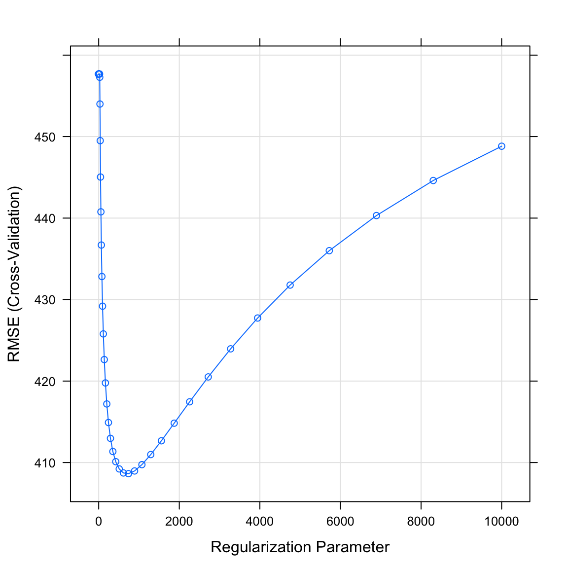
- Print the best value of lambda by running the following code. Does this match what you saw in the plot above?
# Print best regularisation parameter
salary_ridge$bestTune$lambda[1] 739- What were your final regression model coefficients for the best lambda value? Find them by running the following code.
# Get coefficients from best lambda value
coef(salary_ridge$finalModel,
salary_ridge$bestTune$lambda)20 x 1 sparse Matrix of class "dgCMatrix"
1
(Intercept) 608.79
AtBat -8.96
Hits 6.28
HmRun -9.15
Runs 8.39
RBI 6.18
Walks 11.17
Years 12.10
CAtBat 30.42
CHits 32.50
CHmRun 26.36
CRuns 40.55
CRBI 35.48
CWalks 42.49
LeagueN 43.26
DivisionW -42.79
PutOuts 15.77
Assists 41.40
Errors -13.56
NewLeagueN 27.89- How do these coefficients compare to what you found in regular regression? Are they similar? Different?
# Actually the look quite different! The reason why is that we have changed the scale using preProcess
# If you want the coefficients on the original scale, you'd need to convert them, or run your training again without any processing. However, this can lead to problems finding the optimal Lambda value...E - Lasso Regression
It’s time to fit an optimized regression model with a Lasso penalty!
- Before we can fit a lasso regression model, we again first specify which values of the lambda penalty parameter we want to try. Using the code below, create a vector called
lambda_vecwhich contains 100 values between 0 and 1,000.
# Determine possible values of lambda
lambda_vec <- 10 ^ seq(from = -4, to = 4, length = 100)- Fit a lasso regression model predicting
Salaryas a function of all features. Specifically,…
- set the formula to
Salary ~ .. - set the data to
hitters_train. - set the method to
"glmnet"for regularized regression. - set the train control argument to
ctrl_cv. - set the
preProcessargument toc("center", "scale")to make sure the variables are standarised when estimating the beta weights (this is also good practice for lasso regression). - set the tuneGrid argument such that alpha is 1 (for lasso regression), and with all lambda values you specified in
lambda_vec(we’ve done this for you below).
# Lasso Regression --------------------------
salary_lasso <- train(form = XX ~ .,
data = XX,
method = "XX",
trControl = XX,
preProcess = c("XX", "XX"), # Standardise
tuneGrid = expand.grid(alpha = 1, # Lasso penalty
lambda = lambda_vec))# Fit a lasso regression
salary_lasso <- train(form = Salary ~ .,
data = hitters_train,
method = "glmnet",
trControl = ctrl_cv,
preProcess = c("center", "scale"),
tuneGrid = expand.grid(alpha = 1, # Lasso penalty
lambda = lambda_vec))- Print your
salary_lassoobject. What do you see?
salary_lassoglmnet
50 samples
19 predictors
Pre-processing: centered (19), scaled (19)
Resampling: Cross-Validated (10 fold)
Summary of sample sizes: 44, 46, 45, 45, 44, 45, ...
Resampling results across tuning parameters:
lambda RMSE Rsquared MAE
1.00e-04 546 0.222 434
1.20e-04 546 0.222 434
1.45e-04 546 0.222 434
1.75e-04 546 0.222 434
2.10e-04 546 0.222 434
2.54e-04 546 0.222 434
3.05e-04 546 0.222 434
3.68e-04 546 0.222 434
4.43e-04 546 0.222 434
5.34e-04 546 0.222 434
6.43e-04 546 0.222 434
7.74e-04 546 0.222 434
9.33e-04 546 0.222 434
1.12e-03 546 0.222 434
1.35e-03 546 0.222 434
1.63e-03 546 0.222 434
1.96e-03 546 0.222 434
2.36e-03 546 0.222 434
2.85e-03 546 0.222 434
3.43e-03 546 0.222 434
4.13e-03 546 0.222 434
4.98e-03 546 0.222 434
5.99e-03 546 0.222 434
7.22e-03 546 0.222 434
8.70e-03 546 0.222 434
1.05e-02 546 0.222 434
1.26e-02 546 0.222 434
1.52e-02 546 0.222 434
1.83e-02 546 0.222 434
2.21e-02 546 0.222 434
2.66e-02 546 0.222 434
3.20e-02 546 0.222 434
3.85e-02 546 0.222 434
4.64e-02 546 0.223 434
5.59e-02 546 0.223 433
6.73e-02 546 0.224 433
8.11e-02 545 0.224 432
9.77e-02 545 0.225 432
1.18e-01 545 0.226 431
1.42e-01 544 0.227 430
1.71e-01 544 0.229 429
2.06e-01 543 0.231 428
2.48e-01 543 0.234 426
2.98e-01 542 0.237 424
3.59e-01 542 0.241 422
4.33e-01 541 0.245 421
5.21e-01 540 0.251 420
6.28e-01 537 0.258 418
7.56e-01 535 0.264 416
9.11e-01 531 0.262 412
1.10e+00 524 0.257 408
1.32e+00 515 0.258 400
1.59e+00 506 0.258 393
1.92e+00 500 0.264 389
2.31e+00 493 0.284 384
2.78e+00 484 0.318 376
3.35e+00 475 0.355 368
4.04e+00 466 0.374 361
4.86e+00 460 0.378 358
5.86e+00 455 0.373 354
7.05e+00 449 0.361 350
8.50e+00 444 0.369 348
1.02e+01 440 0.375 346
1.23e+01 436 0.388 344
1.48e+01 434 0.402 342
1.79e+01 431 0.418 338
2.15e+01 426 0.434 335
2.60e+01 422 0.451 331
3.13e+01 417 0.468 328
3.76e+01 411 0.488 324
4.53e+01 407 0.501 320
5.46e+01 409 0.516 321
6.58e+01 412 0.526 323
7.92e+01 418 0.529 327
9.55e+01 422 0.526 328
1.15e+02 423 0.516 328
1.38e+02 426 0.491 330
1.67e+02 428 0.483 332
2.01e+02 438 0.483 339
2.42e+02 454 0.450 349
2.92e+02 468 0.152 365
3.51e+02 468 NaN 368
4.23e+02 468 NaN 368
5.09e+02 468 NaN 368
6.14e+02 468 NaN 368
7.39e+02 468 NaN 368
8.90e+02 468 NaN 368
1.07e+03 468 NaN 368
1.29e+03 468 NaN 368
1.56e+03 468 NaN 368
1.87e+03 468 NaN 368
2.26e+03 468 NaN 368
2.72e+03 468 NaN 368
3.27e+03 468 NaN 368
3.94e+03 468 NaN 368
4.75e+03 468 NaN 368
5.72e+03 468 NaN 368
6.89e+03 468 NaN 368
8.30e+03 468 NaN 368
1.00e+04 468 NaN 368
Tuning parameter 'alpha' was held constant at a value of 1
RMSE was used to select the optimal model using the smallest value.
The final values used for the model were alpha = 1 and lambda = 45.3.- Plot your
salary_lassoobject. What do you see? Which value of the regularization parameter seems to be the best?
# Plot salary_lasso object
plot(XX)plot(salary_lasso)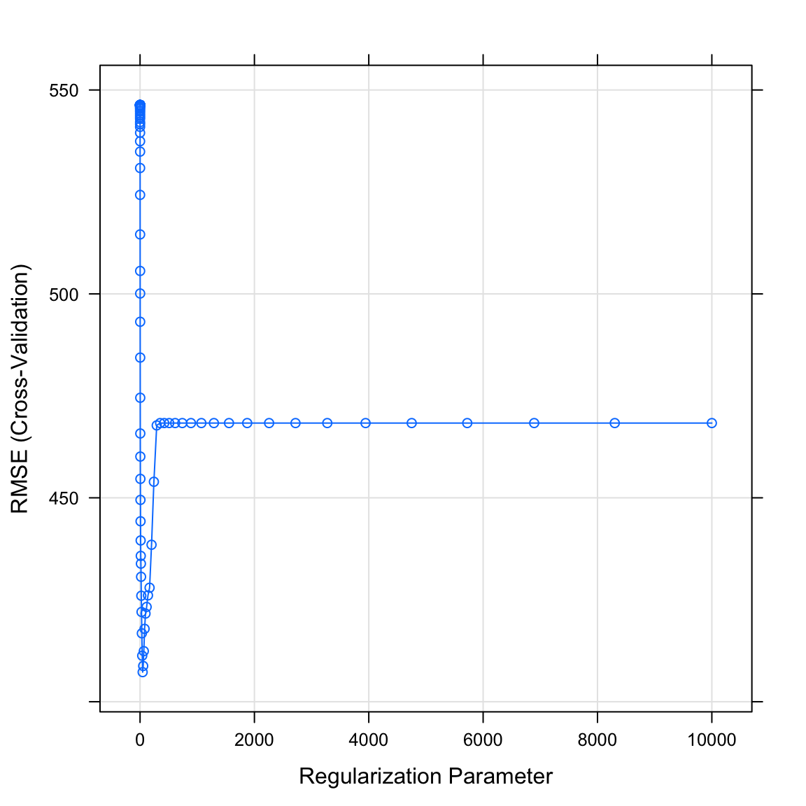
- Print the best value of lambda by running the following code. Does this match what you saw in the plot above?
# Print best regularisation parameter
salary_lasso$bestTune$lambda[1] 45.3- What were your final regression model coefficients for the best lambda value? Find them by running the following code.
# Get coefficients from best lambda value
coef(salary_lasso$finalModel,
salary_lasso$bestTune$lambda)20 x 1 sparse Matrix of class "dgCMatrix"
1
(Intercept) 608.8
AtBat .
Hits .
HmRun .
Runs .
RBI .
Walks .
Years .
CAtBat .
CHits .
CHmRun .
CRuns 134.2
CRBI .
CWalks 108.9
LeagueN 88.9
DivisionW -58.1
PutOuts .
Assists 34.1
Errors .
NewLeagueN . - How do these coefficients compare to what you found in regular regression? Are they similar? Different? Do you notice that any coefficients are now set to exactly 0?
# Yep!
# I see that many features are now removed!F - Decision Tree
It’s time to fit an optimized decision tree model!
- Before we can fit a decision tree, we need to specify which values of the complexity parameter
cpwe want to try. Using the code below, create a vector calledcp_vecwhich contains 100 values between 0 and 1.
# Determine possible values of the complexity parameter cp
cp_vec <- seq(from = 0, to = 1, length = 100)- Fit a decision tree model predicting
Salaryas a function of all features. Specifically,…
- set the formula to
Salary ~ .. - set the data to
hitters_train. - set the method to
"rpart"for decision trees. - set the train control argument to
ctrl_cv, - set the tuneGrid argument with all
cpvalues you specified incp_vec.
# Decision Tree --------------------------
salary_rpart <- train(form = XX ~ .,
data = XX,
method = "XX",
trControl = XX,
tuneGrid = expand.grid(cp = cp_vec))# Decision Tree --------------------------
salary_rpart <- train(form = Salary ~ .,
data = hitters_train,
method = "rpart",
trControl = ctrl_cv,
tuneGrid = expand.grid(cp = cp_vec))- Print your
salary_rpartobject. What do you see?
salary_rpartCART
50 samples
19 predictors
No pre-processing
Resampling: Cross-Validated (10 fold)
Summary of sample sizes: 46, 44, 44, 44, 44, 46, ...
Resampling results across tuning parameters:
cp RMSE Rsquared MAE
0.0000 464 0.3054 354
0.0101 464 0.3054 354
0.0202 464 0.3054 354
0.0303 464 0.3054 354
0.0404 470 0.2618 363
0.0505 470 0.2618 363
0.0606 488 0.2151 384
0.0707 487 0.2010 386
0.0808 487 0.2170 382
0.0909 498 0.2223 395
0.1010 507 0.2092 408
0.1111 508 0.1906 409
0.1212 508 0.1906 409
0.1313 508 0.1906 409
0.1414 503 0.1906 404
0.1515 505 0.1906 411
0.1616 505 0.1906 411
0.1717 505 0.1906 411
0.1818 505 0.1906 411
0.1919 505 0.1906 411
0.2020 505 0.1906 411
0.2121 505 0.1906 411
0.2222 505 0.1906 411
0.2323 505 0.1906 411
0.2424 505 0.1906 411
0.2525 505 0.1906 411
0.2626 505 0.1906 411
0.2727 525 0.1226 423
0.2828 535 0.1255 417
0.2929 535 0.1255 417
0.3030 522 0.0618 409
0.3131 522 0.0618 409
0.3232 522 0.0618 409
0.3333 522 0.0618 409
0.3434 506 0.0320 393
0.3535 506 0.0320 393
0.3636 506 0.0320 393
0.3737 506 0.0320 393
0.3838 506 0.0320 393
0.3939 506 0.0320 393
0.4040 506 0.0320 393
0.4141 506 0.0320 393
0.4242 506 0.0320 393
0.4343 506 0.0320 393
0.4444 506 0.0320 393
0.4545 506 0.0320 393
0.4646 494 NaN 387
0.4747 494 NaN 387
0.4848 494 NaN 387
0.4949 494 NaN 387
0.5051 494 NaN 387
0.5152 494 NaN 387
0.5253 494 NaN 387
0.5354 494 NaN 387
0.5455 494 NaN 387
0.5556 494 NaN 387
0.5657 494 NaN 387
0.5758 494 NaN 387
0.5859 494 NaN 387
0.5960 494 NaN 387
0.6061 494 NaN 387
0.6162 494 NaN 387
0.6263 494 NaN 387
0.6364 494 NaN 387
0.6465 494 NaN 387
0.6566 494 NaN 387
0.6667 494 NaN 387
0.6768 494 NaN 387
0.6869 494 NaN 387
0.6970 494 NaN 387
0.7071 494 NaN 387
0.7172 494 NaN 387
0.7273 494 NaN 387
0.7374 494 NaN 387
0.7475 494 NaN 387
0.7576 494 NaN 387
0.7677 494 NaN 387
0.7778 494 NaN 387
0.7879 494 NaN 387
0.7980 494 NaN 387
0.8081 494 NaN 387
0.8182 494 NaN 387
0.8283 494 NaN 387
0.8384 494 NaN 387
0.8485 494 NaN 387
0.8586 494 NaN 387
0.8687 494 NaN 387
0.8788 494 NaN 387
0.8889 494 NaN 387
0.8990 494 NaN 387
0.9091 494 NaN 387
0.9192 494 NaN 387
0.9293 494 NaN 387
0.9394 494 NaN 387
0.9495 494 NaN 387
0.9596 494 NaN 387
0.9697 494 NaN 387
0.9798 494 NaN 387
0.9899 494 NaN 387
1.0000 494 NaN 387
RMSE was used to select the optimal model using the smallest value.
The final value used for the model was cp = 0.0303.- Plot your
salary_rpartobject. What do you see? Which value of the complexity parameter seems to be the best?
# Plot salary_rpart object
plot(XX)plot(salary_rpart)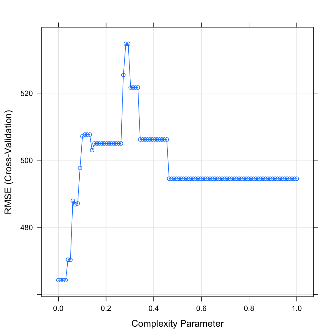
- Print the best value of
cpby running the following code. Does this match what you saw in the plot above?
# Print best regularisation parameter
salary_rpart$bestTune$cp[1] 0.0303- Plot your final decision tree using the following code:
# Visualise your trees
plot(as.party(salary_rpart$finalModel)) 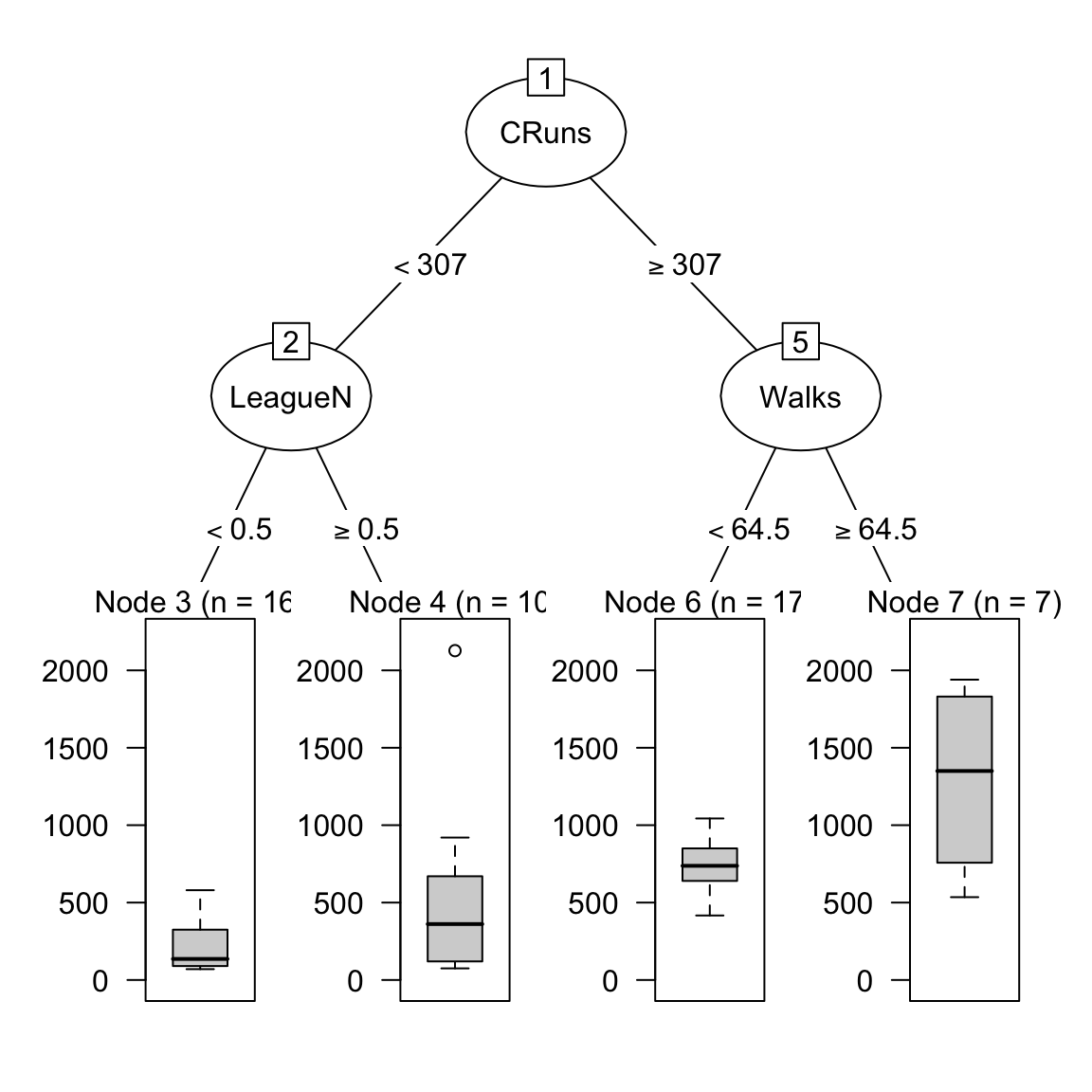
- How do the nodes in the tree compare to the coefficients you found in your regression analyses? Do you see similarities or differences?
# Actually, the tree just has one root and no nodes! This is due to the optimal complexity parameter being so high.G - Random Forests
It’s time to fit an optimized random forest model!
- Before we can fit a random forest model, we need to specify which values of the diversity parameter
mtrywe want to try. Using the code below, create a vector calledmtry_vecwhich is a sequence of numbers from 1 to 10.
# Determine possible values of the random forest diversity parameter mtry
mtry_vec <- 1:10- Fit a random forest model predicting
Salaryas a function of all features. Specifically,…
- set the formula to
Salary ~ .. - set the data to
hitters_train. - set the method to
"rf"for random forests. - set the train control argument to
ctrl_cv. - set the tuneGrid argument such that mtry can take on the values you defined in
mtry_vec.
# Random Forest --------------------------
salary_rf <- train(form = XX ~ .,
data = XX,
method = "XX",
trControl = XX,
tuneGrid = expand.grid(mtry = mtry_vec))# Random Forest --------------------------
salary_rf <- train(form = Salary ~ .,
data = hitters_train,
method = "rf",
trControl = ctrl_cv,
tuneGrid = expand.grid(mtry = mtry_vec))- Print your
salary_rfobject. What do you see?
salary_rfRandom Forest
50 samples
19 predictors
No pre-processing
Resampling: Cross-Validated (10 fold)
Summary of sample sizes: 46, 45, 46, 45, 45, 45, ...
Resampling results across tuning parameters:
mtry RMSE Rsquared MAE
1 353 0.608 259
2 339 0.628 246
3 333 0.634 240
4 331 0.634 240
5 331 0.628 241
6 332 0.630 240
7 331 0.627 239
8 329 0.623 238
9 329 0.623 238
10 328 0.614 238
RMSE was used to select the optimal model using the smallest value.
The final value used for the model was mtry = 10.- Plot your
salary_rfobject. What do you see? Which value of the regularization parameter seems to be the best?
# Plot salary_rf object
plot(XX)plot(salary_rf)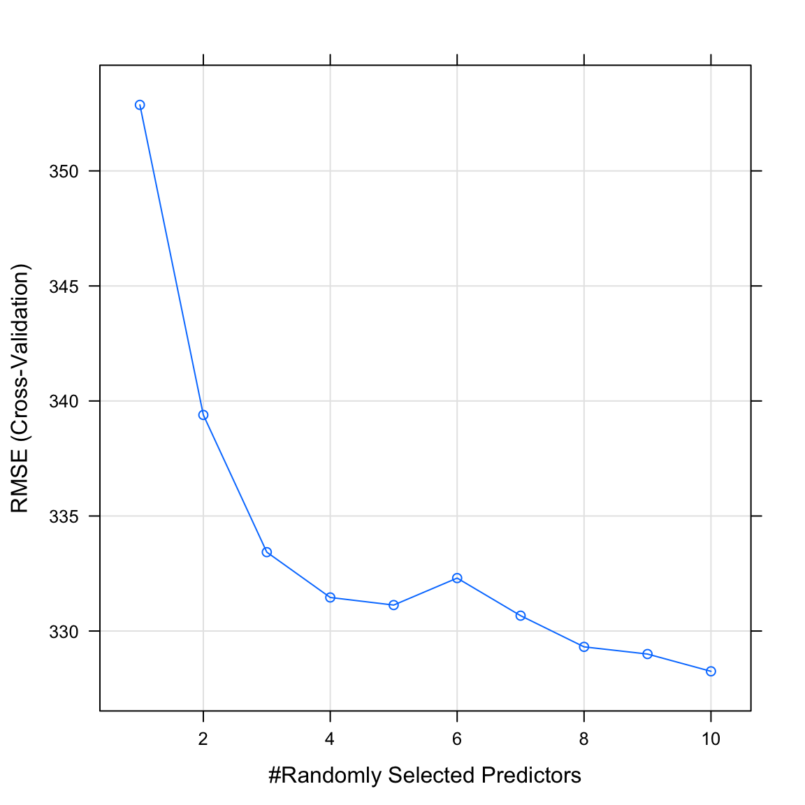
- Print the best value of
mtryby running the following code. Does this match what you saw in the plot above?
# Print best mtry parameter
salary_rf$bestTune$mtry[1] 10H - Estimate prediction accuracy from training folds
- Using
resamples(), calculate the estimated prediction accuracy for each of your models. To do this, put your model objects in the named list (e.g.;glm = salary_glm, …). See below.
# Summarise accuracy statistics across folds
salary_resamples <- resamples(list(glm = XXX,
ridge = XXX,
lasso = XXX,
rpart = XXX,
rf = XXX))# Summarise accuracy statistics across folds
salary_resamples <- resamples(list(glm = salary_glm,
ridge = salary_ridge,
lasso = salary_lasso,
dt = salary_rpart,
rf = salary_rf))- Look at the summary of your
salary_resamplesobject withsummary(salary_resamples). What does this tell you? Which model do you expect to have the best prediction accuracy for the test data?
# Print summaries of cross-validation accuracy
# I see below that the random forest model has the lowest mean MAE, so I
# would expect it to be the best model in the true test data
summary(salary_resamples)
Call:
summary.resamples(object = salary_resamples)
Models: glm, ridge, lasso, dt, rf
Number of resamples: 10
MAE
Min. 1st Qu. Median Mean 3rd Qu. Max. NA's
glm 253 377 497 490 559 743 0
ridge 147 211 319 314 354 596 0
lasso 187 216 297 320 386 514 0
dt 170 262 396 354 423 500 0
rf 45 175 273 238 318 336 0
RMSE
Min. 1st Qu. Median Mean 3rd Qu. Max. NA's
glm 274.8 490 533 575 735 901 0
ridge 176.5 257 387 409 477 916 0
lasso 211.2 233 379 407 458 893 0
dt 267.0 381 429 464 491 812 0
rf 47.2 228 330 328 382 625 0
Rsquared
Min. 1st Qu. Median Mean 3rd Qu. Max. NA's
glm 0.013772 0.1228 0.203 0.377 0.701 0.893 0
ridge 0.131450 0.4330 0.671 0.612 0.808 0.973 0
lasso 0.017893 0.1669 0.581 0.501 0.784 0.965 0
dt 0.000986 0.0235 0.156 0.305 0.463 0.955 0
rf 0.122475 0.3378 0.740 0.614 0.783 0.981 0I - Calculate prediction accuracy
- Save the criterion value for the test data as a new vector called
criterion_test.
# Save salaries of players in test dataset as criterion_test
criterion_test <- XXX$XXXcriterion_test <- hitters_test$Salary- Using
predict(), save the prediction of your regular regression modelsalary_glmfor thehitters_testdata as a new object calledglm_pred. Specifically,…
- set the first argument to
salary_glm. - set the newdata argument to
hitters_test.
# Save the glm predicted salaries of hitters_test
glm_pred <- predict(XXX, newdata = XXX)# Save predictions for glm
glm_pred <- predict(salary_glm, newdata = hitters_test)- Now do the same with your ridge, lasso, decision tree, and random forest models to get the objects
ridge_pred,lasso_pred,rpart_predandrf_pred.
ridge_pred <- predict(XXX, newdata = XXX)
lasso_pred <- predict(XXX, newdata = XXX)
rpart_pred <- predict(XXX, newdata = XXX)
rf_pred <- predict(XXX, newdata = XXX)# Save predictions from other models
ridge_pred <- predict(salary_ridge, newdata = hitters_test)
lasso_pred <- predict(salary_lasso, newdata = hitters_test)
rpart_pred <- predict(salary_rpart, newdata = hitters_test)
rf_pred <- predict(salary_rf, newdata = hitters_test)- Using
postResample(), calculate the aggregate prediction accuracy for each model using the template below. Specifically,…
- set the pred argument to your model predictions (e.g.;
ridge_pred). - set the
obsargument to the true criterion valuescriterion_test).
# Calculate aggregate accuracy for a model
postResample(pred = XXX,
obs = XXX)# Prediction error for normal regression
postResample(pred = glm_pred,
obs = hitters_test$Salary) RMSE Rsquared MAE
552.1782 0.0907 421.8898 # Prediction error for ridge regression
postResample(pred = ridge_pred,
obs = hitters_test$Salary) RMSE Rsquared MAE
366.712 0.329 274.623 # Prediction error for lasso regression
postResample(pred = lasso_pred,
obs = hitters_test$Salary) RMSE Rsquared MAE
389.565 0.254 286.021 # Prediction error for decision trees
postResample(pred = rpart_pred,
obs = hitters_test$Salary) RMSE Rsquared MAE
359.273 0.358 269.471 # Prediction error for random forests
postResample(pred = rf_pred,
obs = hitters_test$Salary) RMSE Rsquared MAE
301.353 0.531 199.995 - Which of your models had the best performance in the true test data?
# Random forests had the lowest test MAE of
postResample(pred = rf_pred,
obs = hitters_test$Salary)[3]MAE
200 - How close were your models’ true prediction error to the values you estimated in the previous section when you ran
resamples()?
# Depends on what you mean by 'close', but they are definitely higher (worse) in the test dataZ - Challenges
- In addition to ‘regular’ 10 fold cross-validation, you can also do repeated 10-fold cross-validation, where the cross validation procedure is repeated many times. Do you think this will improve your models’ performance? To test this, create a new training control object called
ctrl_cv_repas below. Then, train your models again usingctrl_cv_rep(instead ofctrl_cv), and evaluate their prediction performance. Do they improve? Do you get different optimal tuning values compared to your previous models?
# Repeated cross validation.
# Folds = 10
# Repeats = 5
ctrl_cv_rep <- trainControl(method = "repeatedcv",
number = 10,
repeats = 5)Using the same procedure as above, compare models predicting the prices of houses in King County Washington using the
house_trainandhouse_testdatasets.When using lasso regression, do you find that the lasso sets any beta weights to exactly 0? If so, which ones?
Which model does the best and how accurate was it? Was it the same model that performed the best predicting baseball player salaries?
Using the same procedure as above, compare models predicting the graduate rate of students from different colleges using the
college_trainandcollege_testdatasets.When using lasso regression, do you find that the lasso sets any beta weights to exactly 0? If so, which ones?
Which model does the best and how accurate was it? Was it the same model that performed the best predicting baseball player salaries?
Examples
# Model optimization with Regression
# Step 0: Load packages-----------
library(tidyverse) # Load tidyverse for dplyr and tidyr
library(caret) # For ML mastery
library(partykit) # For decision trees
library(party) # For decision trees
# Step 1: Load, clean, and explore data ----------------------
# training data
data_train <- read_csv("1_Data/diamonds_train.csv")
# test data
data_test <- read_csv("1_Data/diamonds_test.csv")
# Convert all characters to factor
# Some ML models require factors
data_train <- data_train %>%
mutate_if(is.character, factor)
data_test <- data_test %>%
mutate_if(is.character, factor)
# Explore training data
data_train # Print the dataset
View(data_train) # Open in a new spreadsheet-like window
dim(data_train) # Print dimensions
names(data_train) # Print the names
# Define criterion_train
# We'll use this later to evaluate model accuracy
criterion_train <- data_train$price
criterion_test <- data_test$price
# Step 2: Define training control parameters -------------
# Use 10-fold cross validation
ctrl_cv <- trainControl(method = "cv",
                        number = 10)
# Step 3: Train models: -----------------------------
# Criterion: hwy
# Features: year, cyl, displ
# Normal Regression --------------------------
price_glm <- train(form = price ~ carat + depth + table + x + y,
data = data_train,
method = "glm",
trControl = ctrl_cv)
# Print key results
price_glm
# RMSE Rsquared MAE
# 1506 0.86 921
# Coefficients
coef(price_glm$finalModel)
# (Intercept) carat depth table x y
# 21464.9 11040.4 -215.6 -94.2 -3681.6 2358.9
# Lasso --------------------------
# Vector of lambda values to try
lambda_vec <- 10 ^ seq(-3, 3, length = 100)
price_lasso <- train(form = price ~ carat + depth + table + x + y,
data = data_train,
method = "glmnet",
trControl = ctrl_cv,
preProcess = c("center", "scale"), # Standardise
tuneGrid = expand.grid(alpha = 1, # Lasso
lambda = lambda_vec))
# Print key results
price_lasso
# glmnet
#
# 5000 samples
# 5 predictor
#
# Pre-processing: centered (5), scaled (5)
# Resampling: Cross-Validated (10 fold)
# Summary of sample sizes: 4500, 4500, 4500, 4500, 4500, 4500, ...
# Resampling results across tuning parameters:
#
# lambda RMSE Rsquared MAE
# 1.00e-03 1509 0.858 918
# 1.15e-03 1509 0.858 918
# 1.32e-03 1509 0.858 918
# 1.52e-03 1509 0.858 918
# Plot regularisation parameter versus error
plot(price_lasso)
# Print best regularisation parameter
price_lasso$bestTune$lambda
# Get coefficients from best lambda value
coef(price_lasso$finalModel,
price_lasso$bestTune$lambda)
# 6 x 1 sparse Matrix of class "dgCMatrix"
# 1
# (Intercept) 4001
# carat 5179
# depth -300
# table -213
# x -3222
# y 1755
# Ridge --------------------------
# Vector of lambda values to try
lambda_vec <- 10 ^ seq(-3, 3, length = 100)
price_ridge <- train(form = price ~ carat + depth + table + x + y,
data = data_train,
method = "glmnet",
trControl = ctrl_cv,
preProcess = c("center", "scale"), # Standardise
tuneGrid = expand.grid(alpha = 0, # Ridge penalty
lambda = lambda_vec))
# Print key results
price_ridge
# glmnet
#
# 5000 samples
# 5 predictor
#
# Pre-processing: centered (5), scaled (5)
# Resampling: Cross-Validated (10 fold)
# Summary of sample sizes: 4500, 4500, 4500, 4500, 4500, 4500, ...
# Resampling results across tuning parameters:
#
# lambda RMSE Rsquared MAE
# 1.00e-03 1638 0.835 1137
# 1.15e-03 1638 0.835 1137
# 1.32e-03 1638 0.835 1137
# 1.52e-03 1638 0.835 1137
# 1.75e-03 1638 0.835 1137
# Plot regularisation parameter versus error
plot(price_ridge)
# Print best regularisation parameter
price_ridge$bestTune$lambda
# Get coefficients from best lambda value
coef(price_ridge$finalModel,
price_ridge$bestTune$lambda)
# 6 x 1 sparse Matrix of class "dgCMatrix"
# 1
# (Intercept) 4001
# carat 2059
# depth -131
# table -168
# x 716
# y 797
# Decision Trees --------------------------
# Vector of cp values to try
cp_vec <- seq(0, .1, length = 100)
price_rpart <- train(form = price ~ carat + depth + table + x + y,
data = data_train,
method = "rpart",
trControl = ctrl_cv,
tuneGrid = expand.grid(cp = cp_vec))
# Print key results
price_rpart
# Plot complexity parameter vs. error
plot(price_rpart)
# Print best complexity parameter
price_rpart$bestTune$cp
# [1] 0.00202
# Step 3: Estimate prediction accuracy from folds ----
# Get accuracy statistics across folds
resamples_price <- resamples(list(ridge = price_ridge,
lasso = price_lasso,
glm = price_glm))
# Print summary of accuracies
summary(resamples_price)
# MAE
# Min. 1st Qu. Median Mean 3rd Qu. Max. NA's
# ridge 1094 1100 1117 1137 1170 1217 0
# lasso 869 887 929 918 944 960 0
# glm 856 882 921 920 949 986 0
#
# RMSE
# Min. 1st Qu. Median Mean 3rd Qu. Max. NA's
# ridge 1545 1580 1609 1638 1703 1772 0
# lasso 1323 1479 1518 1509 1583 1593 0
# glm 1350 1429 1526 1509 1582 1702 0
#
# Rsquared
# Min. 1st Qu. Median Mean 3rd Qu. Max. NA's
# ridge 0.798 0.828 0.836 0.835 0.848 0.854 0
# lasso 0.827 0.846 0.858 0.858 0.868 0.902 0
# glm 0.819 0.849 0.863 0.860 0.870 0.888 0
# Step 4: Measure prediction Accuracy -------------------
# GLM ================================
# Predictions
glm_pred <- predict(price_glm,
newdata = data_test)
# Calculate aggregate accuracy
postResample(pred = glm_pred,
obs = criterion_test)
# RMSE Rsquared MAE
# 1654.017 0.832 944.854
# Ridge ================================
# Predictions
ridge_pred <- predict(price_ridge,
newdata = data_test)
# Calculate aggregate accuracy
postResample(pred = ridge_pred,
obs = criterion_test)
# RMSE Rsquared MAE
# 1650.541 0.832 1133.063
# Lasso ================================
# Predictions
lasso_pred <- predict(price_lasso,
newdata = data_test)
# Calculate aggregate accuracy
postResample(pred = lasso_pred,
obs = criterion_test)
# RMSE Rsquared MAE
# 1653.675 0.832 942.870
# Visualise Accuracy -------------------------
# Tidy competition results
accuracy <- tibble(criterion_test = criterion_test,
Regression = glm_pred,
Ridge = ridge_pred,
Lasso = lasso_pred) %>%
gather(model, prediction, -criterion_test) %>%
# Add error measures
mutate(se = prediction - criterion_test,
ae = abs(prediction - criterion_test))
# Calculate summaries
accuracy_agg <- accuracy %>%
group_by(model) %>%
summarise(mae = mean(ae)) # Calculate MAE (mean absolute error)
# Plot A) Scatterplot of truth versus predictions
ggplot(data = accuracy,
aes(x = criterion_test, y = prediction, col = model)) +
geom_point(alpha = .5) +
geom_abline(slope = 1, intercept = 0) +
labs(x = "True Prices",
y = "Predicted Prices",
title = "Predicting Diamond Prices",
subtitle = "Black line indicates perfect performance")
# Plot B) Violin plot of absolute errors
ggplot(data = accuracy,
aes(x = model, y = ae, fill = model)) +
geom_violin() +
geom_jitter(width = .05, alpha = .2) +
labs(title = "Fitting Absolute Errors",
subtitle = "Numbers indicate means",
x = "Model",
y = "Absolute Error (Log Transformed)") +
guides(fill = FALSE) +
annotate(geom = "label",
x = accuracy_agg$model,
y = accuracy_agg$mae,
label = round(accuracy_agg$mae, 2)) +
scale_y_continuous(trans='log')Datasets
| File | Rows | Columns |
|---|---|---|
| hitters_train.csv | 50 | 20 |
| hitters_test.csv | 213 | 20 |
| college_train.csv | 500 | 18 |
| college_test.csv | 277 | 18 |
| house_train.csv | 5000 | 21 |
| house_test.csv | 1000 | 21 |
The
hitters_trainandhitters_testdata are taken from theHittersdataset in theISLRpackage. They are data frames with observations of major league baseball players from the 1986 and 1987 seasons.The
college_trainandcollege_testdata are taken from theCollegedataset in theISLRpackage. They contain statistics for a large number of US Colleges from the 1995 issue of US News and World Report.The
house_trainandhouse_testdata come from https://www.kaggle.com/harlfoxem/housesalesprediction
Variable description of hitters_train and hitters_test
| Name | Description |
|---|---|
Salary |
1987 annual salary on opening day in thousands of dollars. |
AtBat |
Number of times at bat in 1986. |
Hits |
Number of hits in 1986. |
HmRun |
Number of home runs in 1986. |
Runs |
Number of runs in 1986. |
RBI |
Number of runs batted in in 1986. |
Walks |
Number of walks in 1986. |
Years |
Number of years in the major leagues. |
CAtBat |
Number of times at bat during his career. |
CHits |
Number of hits during his career. |
CHmRun |
Number of home runs during his career. |
CRuns |
Number of runs during his career. |
CRBI |
Number of runs batted in during his career. |
CWalks |
Number of walks during his career. |
League |
A factor with levels A and N indicating player’s league at the end of 1986. |
Division |
A factor with levels E and W indicating player’s division at the end of 1986. |
PutOuts |
Number of put outs in 1986. |
Assists |
Number of assists in 1986. |
Errors |
Number of errors in 1986. |
NewLeague |
A factor with levels A and N indicating player’s league at the beginning of 1987. |
Variable description of college_train and college_test
| Name | Description |
|---|---|
Private |
A factor with levels No and Yes indicating private or public university. |
Apps |
Number of applications received. |
Accept |
Number of applications accepted. |
Enroll |
Number of new students enrolled. |
Top10perc |
Pct. new students from top 10% of H.S. class. |
Top25perc |
Pct. new students from top 25% of H.S. class. |
F.Undergrad |
Number of fulltime undergraduates. |
P.Undergrad |
Number of parttime undergraduates. |
Outstate |
Out-of-state tuition. |
Room.Board |
Room and board costs. |
Books |
Estimated book costs. |
Personal |
Estimated personal spending. |
PhD |
Pct. of faculty with Ph.D.’s. |
Terminal |
Pct. of faculty with terminal degree. |
S.F.Ratio |
Student/faculty ratio. |
perc.alumni |
Pct. alumni who donate. |
Expend |
Instructional expenditure per student. |
Grad.Rate |
Graduation rate. |
Variable description of house_train and house_test
| Name | Description |
|---|---|
price |
Price of the house in $. |
bedrooms |
Number of bedrooms. |
bathrooms |
Number of bathrooms. |
sqft_living |
Square footage of the home. |
sqft_lot |
Square footage of the lot. |
floors |
Total floors (levels) in house. |
waterfront |
House which has a view to a waterfront. |
view |
Has been viewed. |
condition |
How good the condition is (Overall). |
grade |
Overall grade given to the housing unit, based on King County grading system. |
sqft_above |
Square footage of house apart from basement. |
sqft_basement |
Square footage of the basement. |
yr_built |
Built Year. |
yr_renovated |
Year when house was renovated. |
zipcode |
Zip code. |
lat |
Latitude coordinate. |
long |
Longitude coordinate. |
sqft_living15 |
Living room area in 2015 (implies some renovations). This might or might not have affected the lotsize area. |
sqft_lot15 |
lot-size area in 2015 (implies some renovations). |
Functions
Packages
| Package | Installation |
|---|---|
tidyverse |
install.packages("tidyverse") |
caret |
install.packages("caret") |
partykit |
install.packages("partykit") |
party |
install.packages("party") |
Functions
| Function | Package | Description |
|---|---|---|
trainControl() |
caret |
Define modelling control parameters |
train() |
caret |
Train a model |
predict(object, newdata) |
stats |
Predict the criterion values of newdata based on object |
postResample() |
caret |
Calculate aggregate model performance in regression tasks |
confusionMatrix() |
caret |
Calculate aggregate model performance in classification tasks |
Resources
from github.com/rstudio