Prediction

Overview

By the end of this practical you will know how to:

Fit regression, decision trees and random forests to training data.
Evaluate model fitting and prediction performance in a test set.
Compare the fitting and prediction performance of two models.
Explore the effects of features on model predictions.

Tasks

College Graduation Rates

In this section, we will again predict college graduation rates Grad_Rate from the college_train and college_test datasets.

A - Setup

Open your BaselRBootcamp R project. It should already have the folders 1_Data and 2_Code. Make sure that the data file(s) listed in the Datasets section are in your 1_Data folder.
Open a new R script. At the top of the script, using comments, write your name and the date. Save it as a new file called Prediction_College_practical.R in the 2_Code folder.
Using library() load the set of packages for this practical listed in the packages section above.

# Load packages necessary for this script
library(tidyverse)
library(caret)
library(party)
library(partykit)

Run the code below to load each of the datasets listed in the Datasets as new objects.

# College data
college_train <- read_csv(file = "1_Data/college_train.csv")
college_test <- read_csv(file = "1_Data/college_test.csv")

Take a look at the first few rows of each dataframe by printing them to the console.

# Print dataframes to the console
college_train

# A tibble: 500 x 18
   Private  Apps Accept Enroll Top10perc Top25perc F.Undergrad P.Undergrad
   <chr>   <dbl>  <dbl>  <dbl>     <dbl>     <dbl>       <dbl>       <dbl>
 1 Yes      1202   1054    326        18        44        1410         299
 2 Yes      1415    714    338        18        52        1345          44
 3 Yes      4778   2767    678        50        89        2587         120
 4 Yes      1220    974    481        28        67        1964         623
 5 Yes      1981   1541    514        18        36        1927        1084
 6 Yes      1217   1088    496        36        69        1773         884
 7 No       8579   5561   3681        25        50       17880        1673
 8 No        833    669    279         3        13        1224         345
 9 No      10706   7219   2397        12        37       14826        1979
10 Yes       938    864    511        29        62        1715         103
# … with 490 more rows, and 10 more variables: Outstate <dbl>,
#   Room.Board <dbl>, Books <dbl>, Personal <dbl>, PhD <dbl>,
#   Terminal <dbl>, S.F.Ratio <dbl>, perc.alumni <dbl>, Expend <dbl>,
#   Grad.Rate <dbl>

college_test

# A tibble: 277 x 18
   Private  Apps Accept Enroll Top10perc Top25perc F.Undergrad P.Undergrad
   <chr>   <dbl>  <dbl>  <dbl>     <dbl>     <dbl>       <dbl>       <dbl>
 1 No       9251   7333   3076        14        45       13699        1213
 2 Yes      1480   1257    452         6        25        2961         572
 3 No       2336   1725   1043        10        27        5438        4058
 4 Yes      1262   1102    276        14        40         978          98
 5 Yes       959    771    351        23        48        1662         209
 6 Yes       331    331    225        15        36        1100         166
 7 Yes       804    632    281        29        72         840          68
 8 No        285    280    208        21        43        1140         473
 9 Yes       323    278    122        31        51         393           4
10 Yes       504    482    185        10        36         550          84
# … with 267 more rows, and 10 more variables: Outstate <dbl>,
#   Room.Board <dbl>, Books <dbl>, Personal <dbl>, PhD <dbl>,
#   Terminal <dbl>, S.F.Ratio <dbl>, perc.alumni <dbl>, Expend <dbl>,
#   Grad.Rate <dbl>

Print the numbers of rows and columns of each dataset using the dim() function.

# Print numbers of rows and columns
dim(XXX)
dim(XXX)

dim(college_train)

[1] 500  18

dim(college_test)

[1] 277  18

Look at the names of the dataframes with the names() function.

# Print the names of each dataframe
names(XXX)
names(XXX)

names(college_train)

 [1] "Private"     "Apps"        "Accept"      "Enroll"      "Top10perc"  
 [6] "Top25perc"   "F.Undergrad" "P.Undergrad" "Outstate"    "Room.Board" 
[11] "Books"       "Personal"    "PhD"         "Terminal"    "S.F.Ratio"  
[16] "perc.alumni" "Expend"      "Grad.Rate"

names(college_test)

 [1] "Private"     "Apps"        "Accept"      "Enroll"      "Top10perc"  
 [6] "Top25perc"   "F.Undergrad" "P.Undergrad" "Outstate"    "Room.Board" 
[11] "Books"       "Personal"    "PhD"         "Terminal"    "S.F.Ratio"  
[16] "perc.alumni" "Expend"      "Grad.Rate"

Open each dataset in a new window using View(). Do they look ok?

# Open each dataset in a window.
View(XXX)
View(XXX)

Again, We need to do a little bit of data cleaning. Specifically, we need to convert all character columns to factors: Do this by running the following code:

# Convert all character columns to factor
college_train <- college_train %>%
          mutate_if(is.character, factor)

college_test <- college_test %>%
          mutate_if(is.character, factor)

B - Fitting

Your goal in this set of tasks is again to fit models predicting Grad.Rate, the percentage of attendees who graduate from each college.

Using trainControl(), set your training control method to "none". Save your object as ctrl_none.

# Set training method to "none" for simple fitting
#  Note: This is for demonstration purposes, you would almost
#   never do this for a 'real' prediction task!
ctrl_none <- trainControl(method = "XXX")

ctrl_none <- trainControl(method = "none")

Regression

Using train() fit a regression model called grad_glm predicting Grad.Rate as a function of all features. Specifically,…

for the form argument, use Grad.Rate ~ ..
for the data argument, use college_train in the data argument.
for the method argument, use method = "glm" for regression.
for the trControl argument, use your ctrl_none object you created before.

grad_glm <- train(form = XX ~ .,
                  data = XX,
                  method = "XXX",
                  trControl = ctrl_none)

grad_glm <- train(form = Grad.Rate ~ .,
                  data = college_train,
                  method = "glm",
                  trControl = ctrl_none)

Explore your grad_glm object by looking at grad_glm$finalModel and using summary(), what do you find?

grad_glm$XXX
summary(XXX)

grad_glm$finalModel


Call:  NULL

Coefficients:
(Intercept)   PrivateYes         Apps       Accept       Enroll  
  31.010972     1.701840     0.001926    -0.001754     0.005550  
  Top10perc    Top25perc  F.Undergrad  P.Undergrad     Outstate  
  -0.049727     0.206252    -0.001069    -0.001294     0.001782  
 Room.Board        Books     Personal          PhD     Terminal  
   0.000871    -0.000932    -0.001457     0.104743    -0.101789  
  S.F.Ratio  perc.alumni       Expend  
   0.275943     0.219944    -0.000683  

Degrees of Freedom: 499 Total (i.e. Null);  482 Residual
Null Deviance:      142000 
Residual Deviance: 74600    AIC: 3960

summary(grad_glm)


Call:
NULL

Deviance Residuals: 
   Min      1Q  Median      3Q     Max  
-38.10   -7.24   -0.58    7.51   47.10  

Coefficients:
             Estimate Std. Error t value Pr(>|t|)    
(Intercept) 31.010972   5.911481    5.25  2.3e-07 ***
PrivateYes   1.701840   2.114677    0.80  0.42135    
Apps         0.001926   0.000572    3.37  0.00082 ***
Accept      -0.001754   0.001046   -1.68  0.09417 .  
Enroll       0.005550   0.002872    1.93  0.05387 .  
Top10perc   -0.049727   0.086281   -0.58  0.56466    
Top25perc    0.206252   0.066972    3.08  0.00219 ** 
F.Undergrad -0.001069   0.000461   -2.32  0.02068 *  
P.Undergrad -0.001294   0.000444   -2.92  0.00369 ** 
Outstate     0.001782   0.000297    6.01  3.7e-09 ***
Room.Board   0.000871   0.000721    1.21  0.22790    
Books       -0.000932   0.004089   -0.23  0.81988    
Personal    -0.001457   0.000998   -1.46  0.14494    
PhD          0.104743   0.071027    1.47  0.14095    
Terminal    -0.101789   0.076321   -1.33  0.18293    
S.F.Ratio    0.275943   0.191423    1.44  0.15008    
perc.alumni  0.219944   0.061576    3.57  0.00039 ***
Expend      -0.000683   0.000202   -3.39  0.00077 ***
---
Signif. codes:  0 '***' 0.001 '**' 0.01 '*' 0.05 '.' 0.1 ' ' 1

(Dispersion parameter for gaussian family taken to be 155)

    Null deviance: 141641  on 499  degrees of freedom
Residual deviance:  74595  on 482  degrees of freedom
AIC: 3960

Number of Fisher Scoring iterations: 2

Using predict() save the fitted values of grad_glm object as glm_fit.

# Save fitted values of regression model
glm_fit <- predict(XXX)

glm_fit <- predict(grad_glm)

Print your glm_fit object, look at summary statistics with summary(glm_fit), and create a histogram with hist() do they make sense?

# Explore regression model fits
XXX
summary(XXX)
hist(XXX)

glm_fit[1:10]   # Only printing first 10

   1    2    3    4    5    6    7    8    9   10 
71.8 56.4 91.8 62.9 69.2 68.5 57.4 52.0 57.4 71.0

summary(glm_fit)

   Min. 1st Qu.  Median    Mean 3rd Qu.    Max. 
   33.0    57.3    64.1    65.6    73.3   102.8

hist(glm_fit)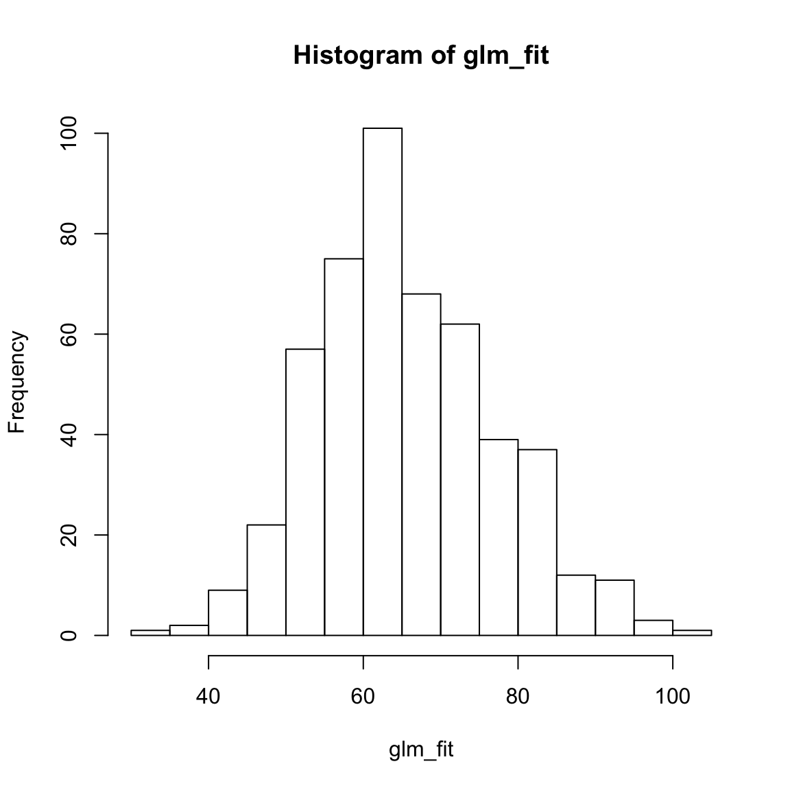

Decision Trees

Using train(), fit a decision tree model called grad_rpart. Specifically,…

for the form argument, use Grad.Rate ~ ..
for the data argument, use college_train.
for the method argument, use method = "rpart" to create decision trees.
for the trControl argument, use your ctrl_none object you created before.
for the tuneGrid argument, use cp = 0.01 to specify the value of the complexity parameter. This is a pretty low value which means your trees will be, relatively, complex, i.e., deep.

grad_rpart <- train(form = XX ~ .,
                  data = XXX,
                  method = "XX",
                  trControl = XX,
                  tuneGrid = expand.grid(cp = XX))   # Set complexity parameter

grad_rpart <- train(form = Grad.Rate ~ .,
                  data = college_train,
                  method = "rpart",
                  trControl = ctrl_none,
                  tuneGrid = expand.grid(cp = .01))   # Set complexity parameter

Explore your grad_rpart object by looking at grad_rpart$finalModel and plotting it with plot(as.party(grad_rpart$finalModel)), what do you find?

grad_rpart$finalModel

n= 500 

node), split, n, deviance, yval
      * denotes terminal node

 1) root 500 142000 65.6  
   2) Outstate< 1.06e+04 292  69000 58.0  
     4) Top25perc< 47.5 135  34100 53.3  
       8) Outstate< 8.56e+03 86  20000 48.9  
        16) Expend>=6.97e+03 26   6430 41.9 *
        17) Expend< 6.97e+03 60  11700 52.0  
          34) Books>=388 53   9310 50.0 *
          35) Books< 388 7    639 66.7 *
       9) Outstate>=8.56e+03 49   9520 61.1 *
     5) Top25perc>=47.5 157  29600 61.9  
      10) Top10perc< 51.5 147  26100 61.0  
        20) perc.alumni< 24.5 110  16700 58.9 *
        21) perc.alumni>=24.5 37   7500 67.2 *
      11) Top10perc>=51.5 10   1570 75.3 *
   3) Outstate>=1.06e+04 208  31500 76.4  
     6) Outstate< 1.68e+04 158  21500 73.3  
      12) perc.alumni< 22.5 55   8180 68.7 *
      13) perc.alumni>=22.5 103  11500 75.8  
        26) F.Undergrad< 1.42e+03 55   4770 71.2 *
        27) F.Undergrad>=1.42e+03 48   4200 81.1 *
     7) Outstate>=1.68e+04 50   4040 85.9 *

plot(as.party(grad_rpart$finalModel))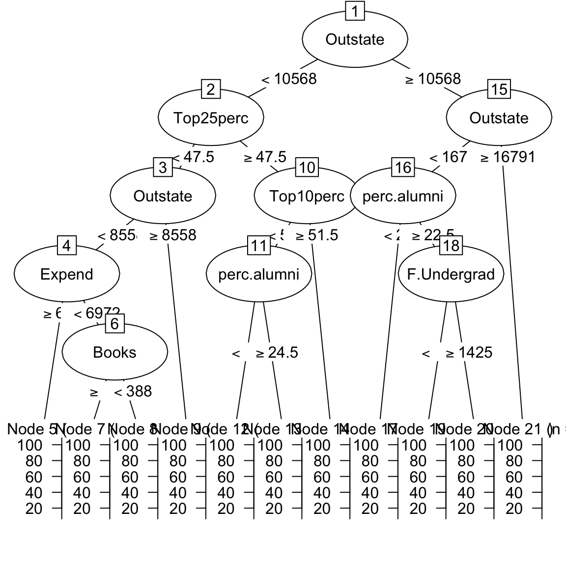

Using predict(), save the fitted values of grad_rpart object as rpart_predfit.

# Save fitted values of decision tree model
rpart_predfit <- predict(XXX)

rpart_predfit <- predict(grad_rpart)

Print your rpart_predfit object, look at summary statistics with summary(rpart_predfit), and create a histogram with hist(). Do they make sense?

# Explore decision tree fits
XXX
summary(XXX)
hist(XXX)

rpart_predfit[1:10] # Only first 10

   1    2    3    4    5    6    7    8    9   10 
71.2 58.9 85.9 58.9 68.7 81.1 58.9 50.0 50.0 81.1

summary(rpart_predfit)

   Min. 1st Qu.  Median    Mean 3rd Qu.    Max. 
   41.9    58.9    67.2    65.6    71.2    85.9

hist(rpart_predfit)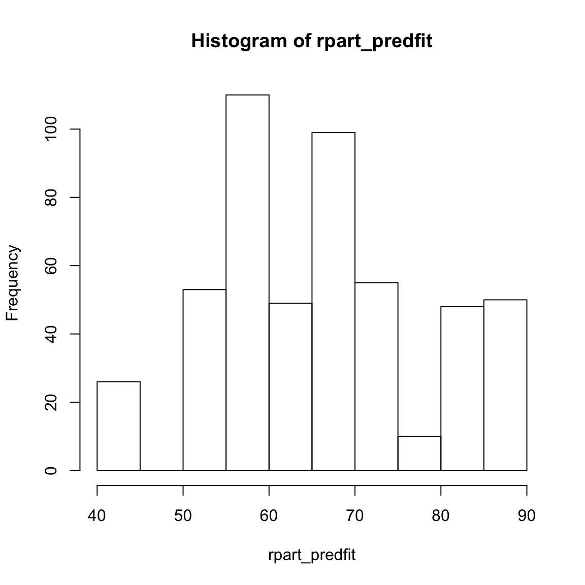

Random Forests

Using train(), fit a random forest model called grad_rf. Speicifically,…

for the form argument, use Grad.Rate ~ ..
for the data argument, use college_train.
for the method argument, use method = "rf" to fit random forests.
for the trControl argument, use your ctrl_none object you created before.
for the mtry parameter, use mtry = 2. This is a relatively low value, so the forest will be very diverse.

grad_rf <- train(form = XX ~ .,   # Predict grad
                 data = XX,
                 method = "XX",
                 trControl = XX,
                 tuneGrid = expand.grid(mtry = XX))  # Set number of features randomly selected

grad_rf <- train(form = Grad.Rate ~ .,   # Predict grad
                 data = college_train,
                 method = "rf",
                 trControl = ctrl_none,
                 tuneGrid = expand.grid(mtry = 2))  # Set number of features randomly selected

Using predict(), save the fitted values of grad_rf object as rf_fit.

# Save fitted values of random forest model
rf_fit <- predict(XXX)

rf_fit <- predict(grad_rf)

Print your rf_fit object, look at summary statistics with summary(rf_fit), and create a histogram with hist(). Do they make sense?

# Explore random forest fits
XXX
summary(XXX)
hist(XXX)

rf_fit[1:10]    # Only first 10

   1    2    3    4    5    6    7    8    9   10 
68.6 64.1 85.1 55.8 76.1 67.3 58.0 43.6 58.5 72.6

summary(rf_fit)

   Min. 1st Qu.  Median    Mean 3rd Qu.    Max. 
   31.4    56.7    65.7    65.6    74.9    96.8

hist(rf_fit)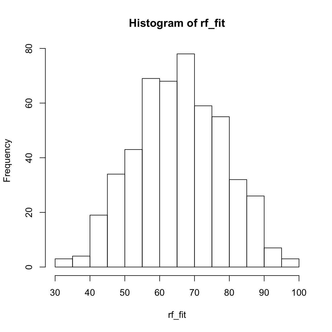

Assess accuracy

Save the true training criterion values (college_train$Grad.Rate) as a vector called criterion_train.

# Save training criterion values
criterion_train <- XXX$XXX

criterion_train <- college_train$Grad.Rate

Using postResample(), determine the fitting performance of each of your models separately. Make sure to set your criterion_train values to the obs argument, and your true model fits XX_fit to the pred argument.

# Calculate fitting accuracies of each model
# pred = XX_fit
# obs = criterion_train

# Regression
postResample(pred = XXX, obs = XXX)

# Decision Trees
postResample(pred = XXX, obs = XXX)

# Random Forests
postResample(pred = XXX, obs = XXX)

# Regression
postResample(pred = glm_fit, obs = criterion_train)

    RMSE Rsquared      MAE 
  12.214    0.473    9.250

# Decision Trees
postResample(pred = rpart_predfit, obs = criterion_train)

    RMSE Rsquared      MAE 
  12.072    0.486    9.536

# Random Forests
postResample(pred = rf_fit, obs = criterion_train)

    RMSE Rsquared      MAE 
   5.736    0.928    4.346

Which one had the best fit? What was the fitting MAE of each model?

(Optional). If you’d like to, try visualizing the fitting results using the plotting code shown in the Examples tab above. Ask for help if you need it!

accuracy <- tibble(criterion_train = criterion_train,
                   Regression = glm_fit,
                   DecisionTrees = rpart_predfit,
                   RandomForest = rf_fit) %>%
               gather(model, prediction, -criterion_train) %>%
               # Add error measures
               mutate(se = prediction - criterion_train,
                      ae = abs(prediction - criterion_train))

# Calculate summaries
accuracy_agg <- accuracy %>%
                  group_by(model) %>%
                  summarise(mae = mean(ae))   # Calculate MAE (mean absolute error)
# Plot A) Scatterplot of truth versus predictions
ggplot(data = accuracy,
       aes(x = criterion_train, y = prediction)) +
  geom_point(alpha = .5) +
  geom_abline(slope = 1, intercept = 0) +
  facet_wrap(~ model) +
  labs(title = "Predicting college_train$Grad.Rate",
       subtitle = "Black line indicates perfect performance")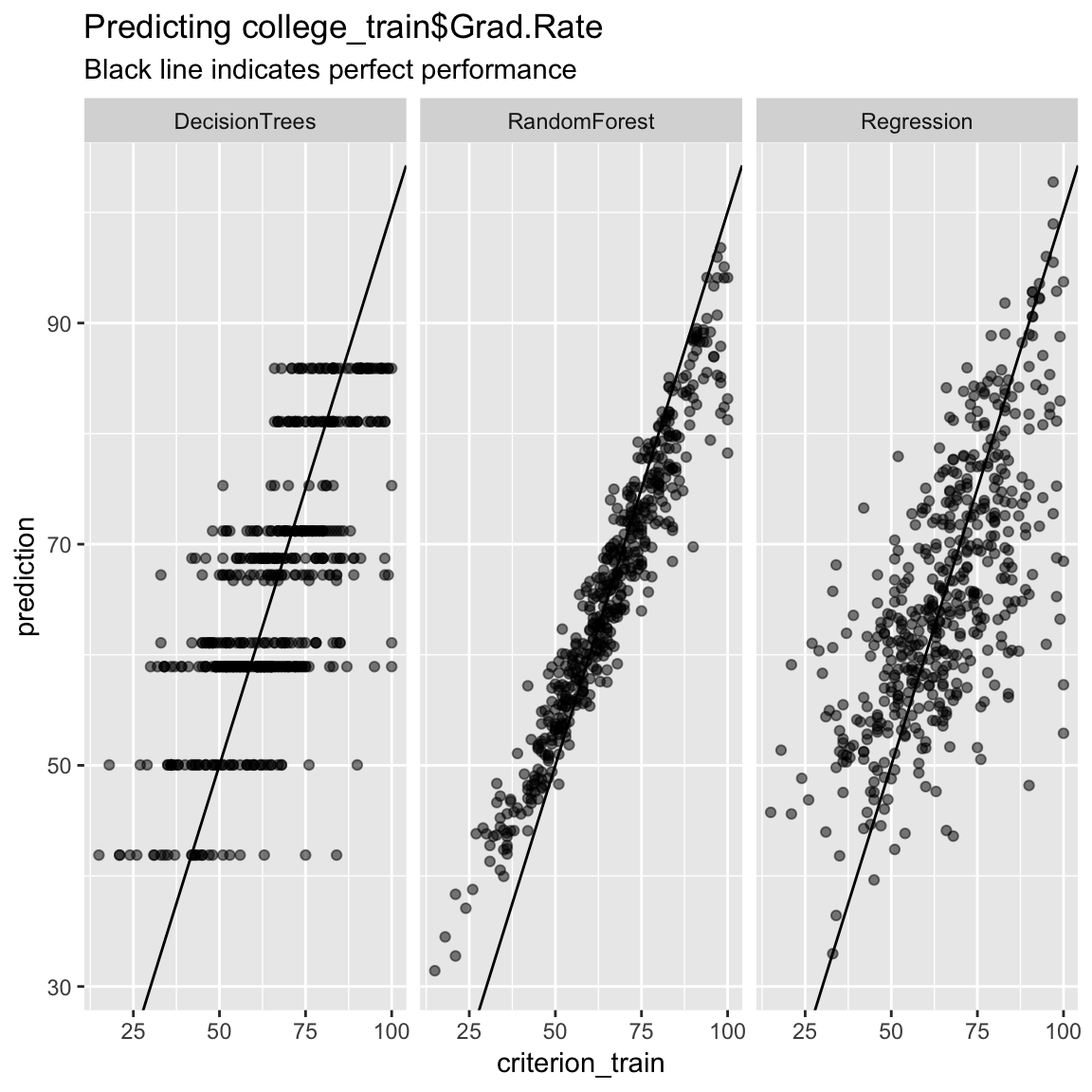

# Plot B) Violin plot of absolute errors
ggplot(data = accuracy, 
       aes(x = model, y = ae, fill = model)) + 
  geom_violin() + 
  geom_jitter(width = .05, alpha = .2) +
  labs(title = "Prediction Absolute Errors",
       subtitle = "Numbers indicate means",
       x = "Model",
       y = "Absolute Error") +
  guides(fill = FALSE) +
  annotate(geom = "label", 
           x = accuracy_agg$model, 
           y = accuracy_agg$mae, 
           label = round(accuracy_agg$mae, 2))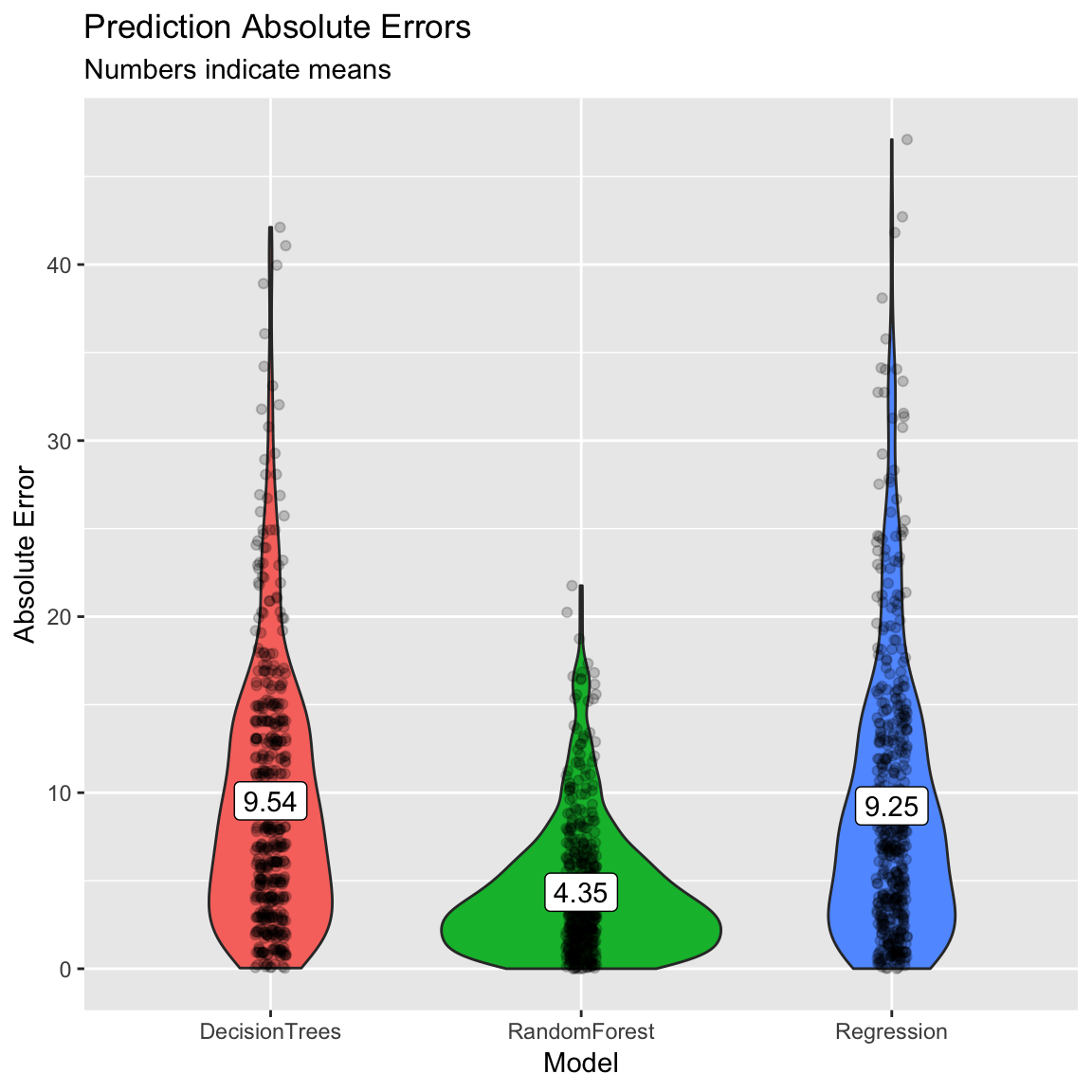

C - Prediction

Save the criterion values from the test data set college_test$Grad.Rate as a new vector called criterion_test.

# Save criterion values
criterion_test <- XXX$XXX

# Save criterion values
criterion_test <- college_test$Grad.Rate

Using predict(), save the predicted values of each model for the test data college_test as glm_pred, rpart_pred and rf_pred.

# Save model predictions for test data
# newdata = college_test

# Regression
glm_pred <- predict(XXX, newdata = XXX)

# Decision Trees
rpart_pred <- predict(XXX, newdata = XXX)

# Random Forests
rf_pred <- predict(XXX, newdata = XXX)

# Save model predictions for test data
# newdata = college_test

# Regression
glm_pred <- predict(grad_glm, newdata = college_test)

# Decision Trees
rpart_pred <- predict(grad_rpart, newdata = college_test)

# Random Forests
rf_pred <- predict(grad_rf, newdata = college_test)

Using postResample(), determine the prediction performance of each of your models against the test criterion criterion_test.

# Calculate prediction accuracies of each model
# obs = criterion_test
# pred = XX_pred

# Regression
postResample(pred = XXX, obs = XXX)

# Decision Trees
postResample(pred = XXX, obs = XXX)

# Random Forests
postResample(pred = XXX, obs = XXX)

# Calculate prediction accuracies of each model
# obs = criterion_test
# pred = XX_pred

# Regression
postResample(pred = glm_pred, obs = criterion_test)

    RMSE Rsquared      MAE 
  13.727    0.404    9.964

# Decision Trees
postResample(pred = rpart_pred, obs = criterion_test)

    RMSE Rsquared      MAE 
  14.741    0.321   11.104

# Random Forests
postResample(pred = rf_pred, obs = criterion_test)

    RMSE Rsquared      MAE 
   13.25     0.46     9.75

How does each model’s prediction or test performance (on the XXX_test data) compare to its fitting or training performance (on the XXX_train data)? Is it worse? Better? The same? What does the change tell you about the models?

# The regression goodness of fit stayed the most constant. The random forest one droped considerably.

Which of the three models has the best prediction performance?

# The random forest predictions are still the most accurate.

If you had to use one of these three models in the real-world, which one would it be? Why?
If someone came to you and asked “If I use your model in the future to predict the graduation rate of a new college, how accurate do you think it would be?”, what would you say?

House Prices in King County, Washington

In this section, we will work with a different data set. Specifically, we will predict the prices of houses in King County Washington (home of Seattle, which you can thank for this) using the house_train and house_test datasets.

D - Setup

Make sure you are still working in your BaselRBootcamp R project, with the folders 1_Data and 2_Code. Make sure that the data file(s) listed in the Datasets section above are in your 1_Data folder
Open a new R script. At the top of the script, using comments, write your name and the date. Save it as a new file called Prediction_HousePrices_practical.R in the 2_Code folder.
Using library() load the set of packages for this practical listed in the packages section above.

# Load packages necessary for this script
library(tidyverse)
library(caret)
library(party)
library(partykit)

Run the code below to load each of the datasets listed in the Datasets as new objects.

# house data
house_train <- read_csv(file = "1_Data/house_train.csv")
house_test <- read_csv(file = "1_Data/house_test.csv")

Take a look at the first few rows of each dataframe by printing them to the console.
Print the numbers of rows and columns of each dataset using the dim() function.

# Print numbers of rows and columns
dim(XXX)
dim(XXX)

Look at the names of the dataframes with the names() function.

# Print the names of each dataframe
names(XXX)
names(XXX)

Open each dataset in a new window using View(). Do they look ok?

# Open each dataset in a window.
View(XXX)
View(XXX)

Again, we need to do a little bit of data cleaning. Convert all character columns to factor.

# Convert all character columns to factor
house_train <- house_train %>%
          mutate_if(is.character, factor)

house_test <- house_test %>%
          mutate_if(is.character, factor)

E - Fitting

Your goal in the following models is to predict price, the selling price of homes in King County WA.

Using trainControl(), set your training control method to "none". Save your object as ctrl_none.

# Set training method to "none" for simple fitting
#  Note: This is for demonstration purposes, you would almost
#   never do this for a 'real' prediction task!
ctrl_none <- trainControl(method = "XXX")

ctrl_none <- trainControl(method = "none")

Regression

Using train(), fit a regression model called price_glm predicting price using all features in house_train. Specifically,…

for the form argument, use price ~ ..
for the data argument, use house_train.
for the method argument, use method = "glm" for regression.
for the trControl argument, use your ctrl_none object you created before.

price_glm <- train(form = XX ~ .,
                  data = XX,
                  method = "XXX",
                  trControl = ctrl_none)

price_glm <- train(form = price ~ .,
                  data = house_train,
                  method = "glm",
                  trControl = ctrl_none)

Explore your price_glm object by looking at price_glm$finalModel and using summary(). What do you find?

price_glm$XXX
summary(XXX)

price_glm$finalModel


Call:  NULL

Coefficients:
  (Intercept)       bedrooms      bathrooms    sqft_living       sqft_lot  
     1.07e+05      -4.64e+04       5.35e+04       1.47e+02       2.31e-01  
       floors     waterfront           view      condition          grade  
     5.03e+03       6.40e+05       5.84e+04       3.03e+04       9.74e+04  
   sqft_above  sqft_basement       yr_built   yr_renovated        zipcode  
     2.40e+01             NA      -2.61e+03       4.31e+00      -5.42e+02  
          lat           long  sqft_living15     sqft_lot15  
     6.14e+05      -2.32e+05       2.71e+01      -2.63e-01  

Degrees of Freedom: 4999 Total (i.e. Null);  4982 Residual
Null Deviance:      6.81e+14 
Residual Deviance: 2.02e+14     AIC: 136000

summary(price_glm)


Call:
NULL

Deviance Residuals: 
     Min        1Q    Median        3Q       Max  
-1114590    -98269    -10834     76308   4063119  

Coefficients: (1 not defined because of singularities)
               Estimate Std. Error t value Pr(>|t|)    
(Intercept)    1.07e+05   6.13e+06    0.02  0.98603    
bedrooms      -4.64e+04   4.14e+03  -11.19  < 2e-16 ***
bathrooms      5.35e+04   7.00e+03    7.65  2.4e-14 ***
sqft_living    1.47e+02   9.33e+00   15.73  < 2e-16 ***
sqft_lot       2.31e-01   1.02e-01    2.26  0.02360 *  
floors         5.03e+03   7.62e+03    0.66  0.50982    
waterfront     6.40e+05   3.53e+04   18.14  < 2e-16 ***
view           5.84e+04   4.52e+03   12.94  < 2e-16 ***
condition      3.03e+04   4.82e+03    6.28  3.6e-10 ***
grade          9.74e+04   4.43e+03   21.99  < 2e-16 ***
sqft_above     2.40e+01   9.25e+00    2.60  0.00935 ** 
sqft_basement        NA         NA      NA       NA    
yr_built      -2.61e+03   1.54e+02  -16.92  < 2e-16 ***
yr_renovated   4.31e+00   7.99e+00    0.54  0.58986    
zipcode       -5.42e+02   6.84e+01   -7.92  3.0e-15 ***
lat            6.14e+05   2.25e+04   27.28  < 2e-16 ***
long          -2.32e+05   2.71e+04   -8.55  < 2e-16 ***
sqft_living15  2.71e+01   7.12e+00    3.81  0.00014 ***
sqft_lot15    -2.63e-01   1.60e-01   -1.64  0.10008    
---
Signif. codes:  0 '***' 0.001 '**' 0.01 '*' 0.05 '.' 0.1 ' ' 1

(Dispersion parameter for gaussian family taken to be 4.06e+10)

    Null deviance: 6.8104e+14  on 4999  degrees of freedom
Residual deviance: 2.0203e+14  on 4982  degrees of freedom
AIC: 136339

Number of Fisher Scoring iterations: 2

Using predict(), save the fitted values of price_glm object as glm_fit.

# Save fitted values of regression model
glm_fit <- predict(XXX)

# Save fitted values of regression model
glm_fit <- predict(price_glm)

Print your glm_fit object, look at summary statistics with summary(glm_fit), and create a histogram with hist(). Do they make sense?

# Explore regression model fits
XXX
summary(XXX)
hist(XXX)

glm_fit[1:10]  # Only first 10

     1      2      3      4      5      6      7      8      9     10 
 47648 276160 927614  95201 553709 590318 669722 581335  -2308 654493

summary(glm_fit)

   Min. 1st Qu.  Median    Mean 3rd Qu.    Max. 
-414135  335260  487481  536998  672715 2821881

hist(glm_fit)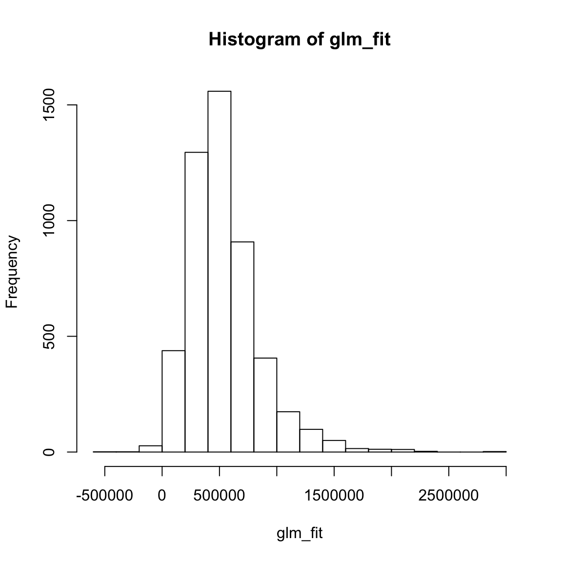

Decision Trees

Using train(), fit a decision tree model called price_rpart predicting price using all features in house_train. Specifically,…

for the form argument, use price ~ ..
for the data argument, use house_train.
for the method argument, use method = "rpart" to create decision trees.
for the trControl argument, use your ctrl_none object you created before.
for the tuneGrid argument, use cp = 0.01 to specify the value of the complexity parameter. This is a pretty low value which means your trees will be, relatively, complex.

price_rpart <- train(form = XX ~ .,
                  data = XXX,
                  method = "XX",
                  trControl = XX,
                  tuneGrid = expand.grid(cp = XX))   # Set complexity parameter

price_rpart <- train(form = price ~ .,
                  data = house_train,
                  method = "rpart",
                  trControl = ctrl_none,
                  tuneGrid = expand.grid(cp = .01))   # Set complexity parameter

Explore your price_rpart object by looking at price_rpart$finalModel and plotting it with plot(as.party(price_rpart$finalModel)). What do you find?

price_rpart$finalModel

n= 5000 

node), split, n, deviance, yval
      * denotes terminal node

 1) root 5000 6.81e+14  537000  
   2) sqft_living< 3.40e+03 4596 2.49e+14  475000  
     4) lat< 47.5 1805 2.85e+13  324000  
       8) sqft_living< 1.95e+03 1075 6.91e+12  268000 *
       9) sqft_living>=1.95e+03 730 1.31e+13  408000 *
     5) lat>=47.5 2791 1.53e+14  572000  
      10) sqft_living< 2.28e+03 1981 5.01e+13  492000  
        20) sqft_living< 1.53e+03 947 1.57e+13  425000 *
        21) sqft_living>=1.53e+03 1034 2.62e+13  554000 *
      11) sqft_living>=2.28e+03 810 5.91e+13  767000  
        22) grade< 8.5 450 1.64e+13  675000 *
        23) grade>=8.5 360 3.39e+13  883000  
          46) long>=-122 237 8.10e+12  774000 *
          47) long< -122 123 1.76e+13 1090000 *
   3) sqft_living>=3.40e+03 404 2.12e+14 1250000  
     6) sqft_living< 6.28e+03 393 1.42e+14 1190000  
      12) waterfront< 0.5 378 1.10e+14 1140000  
        24) grade< 10.5 287 5.38e+13 1010000  
          48) lat< 47.5 65 1.74e+12  626000 *
          49) lat>=47.5 222 3.99e+13 1120000  
            98) long>=-122 119 4.78e+12  922000 *
            99) long< -122 103 2.53e+13 1340000 *
        25) grade>=10.5 91 3.55e+13 1550000  
          50) long>=-122 57 6.47e+12 1250000 *
          51) long< -122 34 1.44e+13 2070000 *
      13) waterfront>=0.5 15 3.52e+12 2550000 *
     7) sqft_living>=6.28e+03 11 2.85e+13 3140000 *

plot(as.party(price_rpart$finalModel))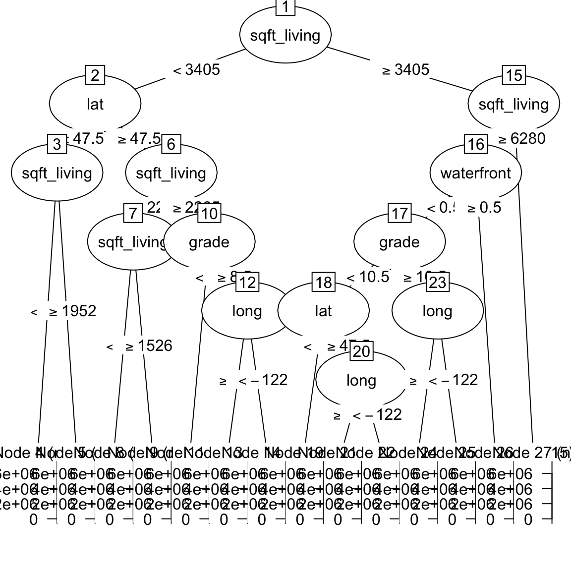

Using predict() save the fitted values of price_rpart object as rpart_predfit.

# Save fitted values of decision tree model
rpart_predfit <- predict(XXX)

rpart_predfit <- predict(price_rpart)

Print your rpart_predfit object, look at summary statistics with summary(rpart_predfit), and create a histogram with hist(). Do they make sense?

# Explore decision tree fits
XXX
summary(XXX)
hist(XXX)

rpart_predfit[1:10]   # Only first 10 values

     1      2      3      4      5      6      7      8      9     10 
267637 267637 921645 267637 553958 553958 407649 553958 267637 674757

summary(rpart_predfit)

   Min. 1st Qu.  Median    Mean 3rd Qu.    Max. 
 267637  407649  424548  536998  553958 3144305

hist(rpart_predfit)

Random Forests

Using train(), fit a random forest model called price_rf predicting price using all features in house_train. Specifically,…

for the form argument, use price ~ ..
for the data argument, use house_train in the data argument.
for the method argument, use method = "rf" to fit random forests.
for the trControl argument, use your ctrl_none object you created before.
for the mtry parameter, use mtry = 2. This is a relatively low value, so the forest will be very diverse.

price_rf <- train(form = XX ~ .,
                 data = XX,
                 method = "XX",
                 trControl = XX,
                 tuneGrid = expand.grid(mtry = XX))  # Set number of features randomly selected

price_rf <- train(form = price ~ .,
                 data = house_train,
                 method = "rf",
                 trControl = ctrl_none,
                 tuneGrid = expand.grid(mtry = 2))  # Set number of features randomly selected

Using predict() save the fitted values of price_rf object as rf_fit.

# Save fitted values of random forest model
rf_fit <- predict(XXX)

rf_fit <- predict(price_rf)

Print your rf_fit object, look at summary statistics with summary(rf_fit), and create a histogram with hist(). Do they make sense?

# Explore random forest fits
XXX
summary(XXX)
hist(XXX)

rf_fit[1:10]   # Only first 10 cases

     1      2      3      4      5      6      7      8      9     10 
193646 350467 843468 155702 557295 630406 641819 446730 216202 674959

summary(rf_fit)

   Min. 1st Qu.  Median    Mean 3rd Qu.    Max. 
 149191  337506  461193  536631  631200 5081078

hist(rf_fit)

Assess accuracy

Save the true training criterion values (house_train$price) as a vector called criterion_train.

# Save training criterion values
criterion_train <- XXX$XXX

criterion_train <- house_train$price

Using postResample(), determine the fitting performance of each of your models separately. Make sure to set your criterion_train values to the obs argument, and your true model fits XX_fit to the pred argument.

# Calculate fitting accuracies of each model
# pred = XX_fit
# obs = criterion_train

# Regression
postResample(pred = XXX, obs = XXX)

# Decision Trees
postResample(pred = XXX, obs = XXX)

# Random Forests
postResample(pred = XXX, obs = XXX)

# Calculate fitting accuracies of each model
# pred = XX_fit
# obs = criterion_train

# Regression
postResample(pred = glm_fit, obs = criterion_train)

    RMSE Rsquared      MAE 
2.01e+05 7.03e-01 1.25e+05

# Decision Trees
postResample(pred = rpart_predfit, obs = criterion_train)

    RMSE Rsquared      MAE 
1.94e+05 7.23e-01 1.19e+05

# Random Forests
postResample(pred = rf_fit, obs = criterion_train)

    RMSE Rsquared      MAE 
7.86e+04 9.67e-01 4.35e+04

Which one had the best fits? What was the fitting MAE of each model?

(Optional). If you’d like to, try visualizing the fitting results using the plotting code shown in the Examples tab above. Ask for help if you need it!

# Tidy competition results
accuracy <- tibble(criterion_train = criterion_train,
                   Regression = glm_fit,
                   DecisionTrees = rpart_predfit,
                   RandomForest = rf_fit) %>%
               gather(model, prediction, -criterion_train) %>%
               # Add error measures
               mutate(se = prediction - criterion_train,
                      ae = abs(prediction - criterion_train))

# Calculate summaries
accuracy_agg <- accuracy %>%
                  group_by(model) %>%
                  summarise(mae = mean(ae))   # Calculate MAE (mean absolute error)

# Plot A) Scatterplot of truth versus predictions
ggplot(data = accuracy,
       aes(x = criterion_train, y = prediction, col = model)) +
  geom_point(alpha = .5) +
  geom_abline(slope = 1, intercept = 0) +
  labs(title = "Predicting Housing Prices",
       subtitle = "Black line indicates perfect performance")

# Plot B) Violin plot of absolute errors
ggplot(data = accuracy, 
       aes(x = model, y = ae, fill = model)) + 
  geom_violin() + 
  geom_jitter(width = .05, alpha = .2) +
  labs(title = "Prediction Absolute Errors",
       subtitle = "Numbers indicate means",
       x = "Model",
       y = "Absolute Error") +
  guides(fill = FALSE) +
  annotate(geom = "label", 
           x = accuracy_agg$model, 
           y = accuracy_agg$mae, 
           label = round(accuracy_agg$mae, 2))

F - Prediction

Save the criterion values from the test data set house_test$price as a new vector called criterion_test.

# Save criterion values
criterion_test <- XXX$XXX

criterion_test <- house_test$price

Using predict(), save the predicted values of each model for the test data house_test as glm_pred, rpart_pred and rf_pred.

# Save model predictions for test data
# object: price_XXX
# newdata: house_test

# Regression
glm_pred <- predict(XXX, newdata = XXX)

# Decision Trees
rpart_pred <- predict(XXX, newdata = XXX)

# Random Forests
rf_pred <- predict(XXX, newdata = XXX)

# Regression
glm_pred <- predict(price_glm, 
                    newdata = house_test)

# Decision Trees
rpart_pred <- predict(price_rpart, 
                      newdata = house_test)

# Random Forests
rf_pred <- predict(price_rf, 
                   newdata = house_test)

Using postResample(), determine the prediction performance of each of your models against the test criterion criterion_test.

# Calculate prediction accuracies of each model
# obs = criterion_test
# pred = XX_pred

# Regression
postResample(pred = XXX, obs = XXX)

# Decision Trees
postResample(pred = XXX, obs = XXX)

# Random Forests
postResample(pred = XXX, obs = XXX)

# Regression
postResample(pred = glm_pred, obs = criterion_test)

    RMSE Rsquared      MAE 
1.92e+05 7.03e-01 1.26e+05

# Decision Trees
postResample(pred = rpart_pred, obs = criterion_test)

    RMSE Rsquared      MAE 
1.84e+05 7.25e-01 1.22e+05

# Random Forests
postResample(pred = rf_pred, obs = criterion_test)

    RMSE Rsquared      MAE 
1.41e+05 8.58e-01 8.05e+04

How does each model’s prediction or test performance (on the XXX_test data) compare to its fitting or training performance (on the XXX_train data)? Is it worse? Better? The same? What does the change tell you about the models?
Which of the three models has the best prediction performance?
If you had to use one of these three models in the real-world, which one would it be? Why?
If someone came to you and asked “If I use your model in the future to predict the price of a new house, how accurate do you think it would be?”, what would you say?

G - Exploring model tuning parameters

In all of your decision tree models so far, you have been setting the complexity parameter to 0.01. Try setting it to a larger value of 0.2 and see how your decision trees change (by plotting them using plot(as.party(XXX_rpart$finalModel))). Do they get more or less complicated? How does increasing this value affect fitting and prediction performance? If you are interested in learning more about this parameter, look at the help menu with ?rpart.control.
In each of your random forest models, you have been setting the mtry argument to 2. Try setting it to a larger value such as 5 and re-run your models. How does increasing this value affect fitting and prediction performance? If you are interested in learning more about this parameter, look at the help menu with ?randomForest.
By default, the train() function uses 500 trees for method = "rf". How do the number of trees affect performance? To answer this, try setting the number of trees to 1,000 (see example below) and re-evaluating your model’s training and test performance. What do you find? What if you set the number of trees to just 10?

# Create random forest model with 1000 trees
mod <- train(form = price ~ .l,
             data = house_train,
             method = "rf",
             trControl = ctrl_none,
             ntree = 1000,   # use 1000 trees! (Instead of the default value of 500)
             tuneGrid = expand.grid(mtry = 2))

Z - Challenges

So far you’ve probably been using most, if not all, available features in predicting house sales. But imagine someone came to you and said "I need to know how much a set of new houses will sell for, but I only have access to three features bedrooms, bathrooms, and sqft_living. Which of your models should I use and how accurate will they be? How would you answer that question? Use your modelling techniques to find out!

price_glm <- train(form = price ~ bedrooms + bathrooms + sqft_living,
                   data = house_train,
                   method = "glm",
                   trControl = ctrl_none)

glm_fit <- predict(price_glm)

price_rpart <- train(form = price ~ bedrooms + bathrooms + sqft_living,
                     data = house_train,
                     method = "rpart",
                     trControl = ctrl_none,
                     tuneGrid = expand.grid(cp = .01))

rpart_predfit <- predict(price_rpart)

price_rf <- train(form = price ~ bedrooms + bathrooms + sqft_living,
                  data = house_train,
                  method = "rf",
                  trControl = ctrl_none,
                  tuneGrid = expand.grid(mtry = 2))

rf_fit <- predict(price_rf)

# Get goodness of fit indices for training set
# Regression
postResample(pred = glm_fit, obs = criterion_train)

    RMSE Rsquared      MAE 
2.63e+05 4.92e-01 1.72e+05

# Decision Trees
postResample(pred = rpart_predfit, obs = criterion_train)

    RMSE Rsquared      MAE 
2.58e+05 5.13e-01 1.69e+05

# Random Forests
postResample(pred = rf_fit, obs = criterion_train)

    RMSE Rsquared      MAE 
1.76e+05 7.82e-01 1.22e+05

# Get predictions

# Regression
glm_pred <- predict(price_glm, 
                    newdata = house_test)

# Decision Trees
rpart_pred <- predict(price_rpart, 
                      newdata = house_test)

# Random Forests
rf_pred <- predict(price_rf, 
                   newdata = house_test)

# Get goodness of fit indices for test sets
# Regression
postResample(pred = glm_pred, obs = criterion_test)

    RMSE Rsquared      MAE 
2.51e+05 4.91e-01 1.68e+05

# Decision Trees
postResample(pred = rpart_pred, obs = criterion_test)

    RMSE Rsquared      MAE 
2.47e+05 5.06e-01 1.64e+05

# Random Forests
postResample(pred = rf_pred, obs = criterion_test)

    RMSE Rsquared      MAE 
2.52e+05 5.01e-01 1.67e+05

Repeat your modelling process, but now do a classification task. Specifically, predict whether or not a house sells for at least $1,000,000. To do this, you’ll first need to create a new column called million in both your house_train and house_test datasets (the code below should help you). Then, use your best modelling techniques to make this prediction. How accurate are your models in predicting whether or not a house will sell for over $1,000,000? Don’t forget to use the confusionMatrix() function instead of postResample() to evaluate your model’s accuracy!

# Add million column to house_train and house_test
#  A factor indicating whether or not a house sells for
#   over 1,000,0000
house_train <- house_train %>%
  mutate(million = factor(price > 1000000))

house_test <- house_test %>%
  mutate(million = factor(price > 1000000))

million_glm <- train(form = million ~ . -price,
                   data = house_train,
                   method = "glm",
                   trControl = ctrl_none)

glm_fit <- predict(million_glm)

million_rpart <- train(form = million ~ . -price,
                     data = house_train,
                     method = "rpart",
                     trControl = ctrl_none,
                     tuneGrid = expand.grid(cp = .01))

rpart_predfit <- predict(million_rpart)

million_rf <- train(form = million ~ . -price,
                  data = house_train,
                  method = "rf",
                  trControl = ctrl_none,
                  tuneGrid = expand.grid(mtry = 2))

rf_fit <- predict(million_rf)

criterion_train <- house_train$million

# Get goodness of fit indices for training set
# Regression
confusionMatrix(data = glm_fit,              # This is the prediction!
                reference = criterion_train) # This is the truth!

Confusion Matrix and Statistics

          Reference
Prediction FALSE TRUE
     FALSE  4618  125
     TRUE     54  203
                                        
               Accuracy : 0.964         
                 95% CI : (0.959, 0.969)
    No Information Rate : 0.934         
    P-Value [Acc > NIR] : < 2e-16       
                                        
                  Kappa : 0.675         
                                        
 Mcnemar's Test P-Value : 1.68e-07      
                                        
            Sensitivity : 0.988         
            Specificity : 0.619         
         Pos Pred Value : 0.974         
         Neg Pred Value : 0.790         
             Prevalence : 0.934         
         Detection Rate : 0.924         
   Detection Prevalence : 0.949         
      Balanced Accuracy : 0.804         
                                        
       'Positive' Class : FALSE

# Decision Trees
confusionMatrix(data = rpart_predfit,        # This is the prediction!
                reference = criterion_train) # This is the truth!

Confusion Matrix and Statistics

          Reference
Prediction FALSE TRUE
     FALSE  4609   72
     TRUE     63  256
                                        
               Accuracy : 0.973         
                 95% CI : (0.968, 0.977)
    No Information Rate : 0.934         
    P-Value [Acc > NIR] : <2e-16        
                                        
                  Kappa : 0.777         
                                        
 Mcnemar's Test P-Value : 0.491         
                                        
            Sensitivity : 0.987         
            Specificity : 0.780         
         Pos Pred Value : 0.985         
         Neg Pred Value : 0.803         
             Prevalence : 0.934         
         Detection Rate : 0.922         
   Detection Prevalence : 0.936         
      Balanced Accuracy : 0.884         
                                        
       'Positive' Class : FALSE

# Random Forests
confusionMatrix(data = rf_fit,               # This is the prediction!
                reference = criterion_train) # This is the truth!

Confusion Matrix and Statistics

          Reference
Prediction FALSE TRUE
     FALSE  4672    0
     TRUE      0  328
                                    
               Accuracy : 1         
                 95% CI : (0.999, 1)
    No Information Rate : 0.934     
    P-Value [Acc > NIR] : <2e-16    
                                    
                  Kappa : 1         
                                    
 Mcnemar's Test P-Value : NA        
                                    
            Sensitivity : 1.000     
            Specificity : 1.000     
         Pos Pred Value : 1.000     
         Neg Pred Value : 1.000     
             Prevalence : 0.934     
         Detection Rate : 0.934     
   Detection Prevalence : 0.934     
      Balanced Accuracy : 1.000     
                                    
       'Positive' Class : FALSE

# Get predictions

# Regression
glm_pred <- predict(million_glm, 
                    newdata = house_test)

# Decision Trees
rpart_pred <- predict(million_rpart, 
                      newdata = house_test)

# Random Forests
rf_pred <- predict(million_rf, 
                   newdata = house_test)

# Get goodness of fit indices for test sets

# create test criterion
criterion_test <- house_test$million
# Regression
confusionMatrix(data = glm_pred,            # This is the prediction!
                reference = criterion_test) # This is the truth!

Confusion Matrix and Statistics

          Reference
Prediction FALSE TRUE
     FALSE   927   23
     TRUE     10   40
                                        
               Accuracy : 0.967         
                 95% CI : (0.954, 0.977)
    No Information Rate : 0.937         
    P-Value [Acc > NIR] : 1.49e-05      
                                        
                  Kappa : 0.691         
                                        
 Mcnemar's Test P-Value : 0.0367        
                                        
            Sensitivity : 0.989         
            Specificity : 0.635         
         Pos Pred Value : 0.976         
         Neg Pred Value : 0.800         
             Prevalence : 0.937         
         Detection Rate : 0.927         
   Detection Prevalence : 0.950         
      Balanced Accuracy : 0.812         
                                        
       'Positive' Class : FALSE

# Decision Trees
confusionMatrix(data = rpart_pred,          # This is the prediction!
                reference = criterion_test) # This is the truth!

Confusion Matrix and Statistics

          Reference
Prediction FALSE TRUE
     FALSE   923   14
     TRUE     14   49
                                       
               Accuracy : 0.972        
                 95% CI : (0.96, 0.981)
    No Information Rate : 0.937        
    P-Value [Acc > NIR] : 3.14e-07     
                                       
                  Kappa : 0.763        
                                       
 Mcnemar's Test P-Value : 1            
                                       
            Sensitivity : 0.985        
            Specificity : 0.778        
         Pos Pred Value : 0.985        
         Neg Pred Value : 0.778        
             Prevalence : 0.937        
         Detection Rate : 0.923        
   Detection Prevalence : 0.937        
      Balanced Accuracy : 0.881        
                                       
       'Positive' Class : FALSE

# Random Forests
confusionMatrix(data = rf_pred,             # This is the prediction!
                reference = criterion_test) # This is the truth!

Confusion Matrix and Statistics

          Reference
Prediction FALSE TRUE
     FALSE   936   27
     TRUE      1   36
                                       
               Accuracy : 0.972        
                 95% CI : (0.96, 0.981)
    No Information Rate : 0.937        
    P-Value [Acc > NIR] : 3.14e-07     
                                       
                  Kappa : 0.706        
                                       
 Mcnemar's Test P-Value : 2.31e-06     
                                       
            Sensitivity : 0.999        
            Specificity : 0.571        
         Pos Pred Value : 0.972        
         Neg Pred Value : 0.973        
             Prevalence : 0.937        
         Detection Rate : 0.936        
   Detection Prevalence : 0.963        
      Balanced Accuracy : 0.785        
                                       
       'Positive' Class : FALSE

Examples

# Fitting and evaluating regression, decision trees, and random forests

# Step 0: Load packages-----------
library(tidyverse)    # Load tidyverse for dplyr and tidyr
library(caret)        # For ML mastery 
library(partykit)     # For decision trees
library(party)        # For decision trees

# Step 1: Load and Clean, and Explore Training data ----------------------

# training data
data_train <- read_csv("1_Data/mpg_train.csv")

# test data
data_test <- read_csv("1_Data/mpg_test.csv")

# Convert all characters to factor
#  Some ML models require factors
data_train <- data_train %>%
  mutate_if(is.character, factor)

data_test <- data_test %>%
  mutate_if(is.character, factor)

# Explore training data
data_train        # Print the dataset
View(data_train)  # Open in a new spreadsheet-like window 
dim(data_train)   # Print dimensions
names(data_train) # Print the names

# Define criterion_train
#   We'll use this later to evaluate model accuracy
criterion_train <- data_train$hwy

# Step 2: Define training control parameters -------------

# In this case, I will set method = "none" to fit to 
#  the entire dataset without any fancy methods
ctrl_none <- trainControl(method = "none") 

# Step 3: Train model: -----------------------------
#   Criterion: hwy
#   Features: year, cyl, displ

# Regression --------------------------
hwy_glm <- train(form = hwy ~ year + cyl + displ,
                 data = data_train,
                 method = "glm",
                 trControl = ctrl_none)

# Look at summary information
hwy_glm$finalModel
summary(hwy_glm)

# Save fitted values
glm_fit <- predict(hwy_glm)

#  Calculate fitting accuracies
postResample(pred = glm_fit, 
             obs = criterion_train)

# Decision Trees ----------------
hwy_rpart <- train(form = hwy ~ year + cyl + displ,
                data = data_train,
                method = "rpart",
                trControl = ctrl_none,
                tuneGrid = expand.grid(cp = .01))   # Set complexity parameter

# Look at summary information
hwy_rpart$finalModel
plot(as.party(hwy_rpart$finalModel))   # Visualise your trees

# Save fitted values
rpart_predfit <- predict(hwy_rpart)

# Calculate fitting accuracies
postResample(pred = rpart_predfit, obs = criterion_train)

# Random Forests -------------------------
hwy_rf <- train(form = hwy ~ year + cyl + displ,
                data = data_train,
                method = "rf",
                trControl = ctrl_none,
                tuneGrid = expand.grid(mtry = 2))   # Set number of features randomly selected

# Look at summary information
hwy_rf$finalModel

# Save fitted values
rf_fit <- predict(hwy_rf)

# Calculate fitting accuracies
postResample(pred = rf_fit, obs = criterion_train)

# Visualise Accuracy -------------------------

# Tidy competition results
accuracy <- tibble(criterion_train = criterion_train,
                   Regression = glm_fit,
                   DecisionTrees = rpart_predfit,
                   RandomForest = rf_fit) %>%
               gather(model, prediction, -criterion_train) %>%
               # Add error measures
               mutate(se = prediction - criterion_train,
                      ae = abs(prediction - criterion_train))

# Calculate summaries
accuracy_agg <- accuracy %>%
                  group_by(model) %>%
                  summarise(mae = mean(ae))   # Calculate MAE (mean absolute error)

# Plot A) Scatterplot of truth versus predictions
ggplot(data = accuracy,
       aes(x = criterion_train, y = prediction, col = model)) +
  geom_point(alpha = .5) +
  geom_abline(slope = 1, intercept = 0) +
  labs(title = "Predicting mpg$hwy",
       subtitle = "Black line indicates perfect performance")

# Plot B) Violin plot of absolute errors
ggplot(data = accuracy, 
       aes(x = model, y = ae, fill = model)) + 
  geom_violin() + 
  geom_jitter(width = .05, alpha = .2) +
  labs(title = "Fitting Absolute Errors",
       subtitle = "Numbers indicate means",
       x = "Model",
       y = "Absolute Error") +
  guides(fill = FALSE) +
  annotate(geom = "label", 
           x = accuracy_agg$model, 
           y = accuracy_agg$mae, 
           label = round(accuracy_agg$mae, 2))

# Step 5: Access prediction ------------------------------

# Define criterion_train
criterion_test <- data_test$hwy

# Save predicted values
glm_pred <- predict(hwy_glm, newdata = data_test)
rpart_pred <- predict(hwy_rpart, newdata = data_test)
rf_pred <- predict(hwy_rf, newdata = data_test)

#  Calculate fitting accuracies
postResample(pred = glm_pred, obs = criterion_test)
postResample(pred = rpart_pred, obs = criterion_test)
postResample(pred = rf_pred, obs = criterion_test)

# Visualise Accuracy -------------------------

# Tidy competition results
accuracy <- tibble(criterion_test = criterion_test,
                   Regression = glm_pred,
                   DecisionTrees = rpart_pred,
                   RandomForest = rf_pred) %>%
               gather(model, prediction, -criterion_test) %>%
               # Add error measures
               mutate(se = prediction - criterion_test,
                      ae = abs(prediction - criterion_test))

# Calculate summaries
accuracy_agg <- accuracy %>%
                  group_by(model) %>%
                  summarise(mae = mean(ae))   # Calculate MAE (mean absolute error)

# Plot A) Scatterplot of truth versus predictions
ggplot(data = accuracy,
       aes(x = criterion_test, y = prediction, col = model)) +
  geom_point(alpha = .5) +
  geom_abline(slope = 1, intercept = 0) +
  labs(title = "Predicting mpg$hwy",
       subtitle = "Black line indicates perfect performance")

# Plot B) Violin plot of absolute errors
ggplot(data = accuracy, 
       aes(x = model, y = ae, fill = model)) + 
  geom_violin() + 
  geom_jitter(width = .05, alpha = .2) +
  labs(title = "Prediction Absolute Errors",
       subtitle = "Numbers indicate means",
       x = "Model",
       y = "Absolute Error") +
  guides(fill = FALSE) +
  annotate(geom = "label", 
           x = accuracy_agg$model, 
           y = accuracy_agg$mae, 
           label = round(accuracy_agg$mae, 2))

Datasets

File	Rows	Columns
college_train.csv	500	18
college_test.csv	277	18
house_train.csv	5000	21
house_test.csv	1000	21

The college_train and college_test data are taken from the College dataset in the ISLR package. They contain statistics for a large number of US Colleges from the 1995 issue of US News and World Report.
The house_train and house_test data come from https://www.kaggle.com/harlfoxem/housesalesprediction

Variable description of `college_train` and `college_test`

Name	Description
`Private`	A factor with levels No and Yes indicating private or public university.
`Apps`	Number of applications received.
`Accept`	Number of applications accepted.
`Enroll`	Number of new students enrolled.
`Top10perc`	Pct. new students from top 10% of H.S. class.
`Top25perc`	Pct. new students from top 25% of H.S. class.
`F.Undergrad`	Number of fulltime undergraduates.
`P.Undergrad`	Number of parttime undergraduates.
`Outstate`	Out-of-state tuition.
`Room.Board`	Room and board costs.
`Books`	Estimated book costs.
`Personal`	Estimated personal spending.
`PhD`	Pct. of faculty with Ph.D.’s.
`Terminal`	Pct. of faculty with terminal degree.
`S.F.Ratio`	Student/faculty ratio.
`perc.alumni`	Pct. alumni who donate.
`Expend`	Instructional expenditure per student.
`Grad.Rate`	Graduation rate.

Variable description of `house_train` and `house_test`

Name	Description
`price`	Price of the house in $.
`bedrooms`	Number of bedrooms.
`bathrooms`	Number of bathrooms.
`sqft_living`	Square footage of the home.
`sqft_lot`	Square footage of the lot.
`floors`	Total floors (levels) in house.
`waterfront`	House which has a view to a waterfront.
`view`	Has been viewed.
`condition`	How good the condition is (Overall).
`grade`	Overall grade given to the housing unit, based on King County grading system.
`sqft_above`	Square footage of house apart from basement.
`sqft_basement`	Square footage of the basement.
`yr_built`	Built Year.
`yr_renovated`	Year when house was renovated.
`zipcode`	Zip code.
`lat`	Latitude coordinate.
`long`	Longitude coordinate.
`sqft_living15`	Living room area in 2015 (implies some renovations). This might or might not have affected the lotsize area.
`sqft_lot15`	lot-size area in 2015 (implies some renovations).

Functions

Packages

Package	Installation
`tidyverse`	`install.packages("tidyverse")`
`caret`	`install.packages("caret")`
`partykit`	`install.packages("partykit")`
`party`	`install.packages("party")`

Functions

Function	Package	Description
`trainControl()`	`caret`	Define modelling control parameters
`train()`	`caret`	Train a model
`predict(object, newdata)`	`stats`	Predict the criterion values of `newdata` based on `object`
`postResample()`	`caret`	Calculate aggregate model performance in regression tasks
`confusionMatrix()`	`caret`	Calculate aggregate model performance in classification tasks

Resources

Cheatsheet

Prediction

Machine Learning with R Basel R Bootcamp

Overview

Tasks

College Graduation Rates

A - Setup

B - Fitting

Regression

Decision Trees

Random Forests

Assess accuracy

C - Prediction

House Prices in King County, Washington

D - Setup

E - Fitting

Regression

Decision Trees

Random Forests

Assess accuracy

F - Prediction

G - Exploring model tuning parameters

Z - Challenges

Examples

Datasets

Variable description of college_train and college_test

Variable description of house_train and house_test

Functions

Packages

Functions

Resources

Cheatsheet

Machine Learning with R
Basel R Bootcamp

Variable description of `college_train` and `college_test`

Variable description of `house_train` and `house_test`