Analysing
R for Data Science
Basel R Bootcamp

Basel R Bootcamp

adapted from trueloveproperty.co.uk
Overview
In this practical, you’ll practice grouping and analysing data with dplyr
By the end of this practical you will know how to:
- Group data and calculate summary statistics
- Run statistical analyses with the generalised linear model.
Tasks
A - Setup
- Open your
BaselRBootcampR project. It should already have the folders1_Dataand2_Code. Make sure that the data files listed in theDatasetssection above are in your1_Datafolder.
# Done!- Open a new R script. At the top of the script, using comments, write your name and the date and “Analysing Practical”.
## NAME
## DATE
## Analysing Practical
Save it as a new file called
analysing_practical.Rin the2_Codefolder.Using
library()load thetidyverseandbroompackages for this practical listed in the Functions section above. If you don’t have them installed, you’ll need to install them, see the Functions tab above for installation instructions.
# Load packages
library(tidyverse)
library(broom)
library(tidyverse)
library(broom)- For this practical, we’ll use the
kc_house.csvdata. This dataset contains house sale prices for King County, Washington. It includes homes sold between May 2014 and May 2015. Using the following template, load the data into R and store it as a new object calledkc_house.
kc_house <- read_csv(file = "XX/XX")- Using
print(),dim(),summary(),head(), andView(), explore the data to make sure it was loaded correctly.
kc_house# A tibble: 21,613 x 21
id date price bedrooms bathrooms sqft_living sqft_lot
<chr> <dttm> <dbl> <dbl> <dbl> <dbl> <dbl>
1 7129… 2014-10-13 00:00:00 2.22e5 3 1 1180 5650
2 6414… 2014-12-09 00:00:00 5.38e5 3 2.25 2570 7242
3 5631… 2015-02-25 00:00:00 1.80e5 2 1 770 10000
4 2487… 2014-12-09 00:00:00 6.04e5 4 3 1960 5000
5 1954… 2015-02-18 00:00:00 5.10e5 3 2 1680 8080
6 7237… 2014-05-12 00:00:00 1.23e6 4 4.5 5420 101930
7 1321… 2014-06-27 00:00:00 2.58e5 3 2.25 1715 6819
8 2008… 2015-01-15 00:00:00 2.92e5 3 1.5 1060 9711
9 2414… 2015-04-15 00:00:00 2.30e5 3 1 1780 7470
10 3793… 2015-03-12 00:00:00 3.23e5 3 2.5 1890 6560
# … with 21,603 more rows, and 14 more variables: floors <dbl>,
# waterfront <dbl>, view <dbl>, condition <dbl>, grade <dbl>,
# sqft_above <dbl>, sqft_basement <dbl>, yr_built <dbl>,
# yr_renovated <dbl>, zipcode <dbl>, lat <dbl>, long <dbl>,
# sqft_living15 <dbl>, sqft_lot15 <dbl>dim(kc_house)[1] 21613 21summary(kc_house) id date price
Length:21613 Min. :2014-05-02 00:00:00 Min. : 75000
Class :character 1st Qu.:2014-07-22 00:00:00 1st Qu.: 321950
Mode :character Median :2014-10-16 00:00:00 Median : 450000
Mean :2014-10-29 04:38:01 Mean : 540088
3rd Qu.:2015-02-17 00:00:00 3rd Qu.: 645000
Max. :2015-05-27 00:00:00 Max. :7700000
bedrooms bathrooms sqft_living sqft_lot
Min. : 0.0 Min. :0.00 Min. : 290 Min. : 520
1st Qu.: 3.0 1st Qu.:1.75 1st Qu.: 1427 1st Qu.: 5040
Median : 3.0 Median :2.25 Median : 1910 Median : 7618
Mean : 3.4 Mean :2.11 Mean : 2080 Mean : 15107
3rd Qu.: 4.0 3rd Qu.:2.50 3rd Qu.: 2550 3rd Qu.: 10688
Max. :33.0 Max. :8.00 Max. :13540 Max. :1651359
floors waterfront view condition
Min. :1.00 Min. :0.000 Min. :0.00 Min. :1.00
1st Qu.:1.00 1st Qu.:0.000 1st Qu.:0.00 1st Qu.:3.00
Median :1.50 Median :0.000 Median :0.00 Median :3.00
Mean :1.49 Mean :0.008 Mean :0.23 Mean :3.41
3rd Qu.:2.00 3rd Qu.:0.000 3rd Qu.:0.00 3rd Qu.:4.00
Max. :3.50 Max. :1.000 Max. :4.00 Max. :5.00
grade sqft_above sqft_basement yr_built
Min. : 1.00 Min. : 290 Min. : 0 Min. :1900
1st Qu.: 7.00 1st Qu.:1190 1st Qu.: 0 1st Qu.:1951
Median : 7.00 Median :1560 Median : 0 Median :1975
Mean : 7.66 Mean :1788 Mean : 292 Mean :1971
3rd Qu.: 8.00 3rd Qu.:2210 3rd Qu.: 560 3rd Qu.:1997
Max. :13.00 Max. :9410 Max. :4820 Max. :2015
yr_renovated zipcode lat long
Min. : 0 Min. :98001 Min. :47.2 Min. :-122
1st Qu.: 0 1st Qu.:98033 1st Qu.:47.5 1st Qu.:-122
Median : 0 Median :98065 Median :47.6 Median :-122
Mean : 84 Mean :98078 Mean :47.6 Mean :-122
3rd Qu.: 0 3rd Qu.:98118 3rd Qu.:47.7 3rd Qu.:-122
Max. :2015 Max. :98199 Max. :47.8 Max. :-121
sqft_living15 sqft_lot15
Min. : 399 Min. : 651
1st Qu.:1490 1st Qu.: 5100
Median :1840 Median : 7620
Mean :1987 Mean : 12768
3rd Qu.:2360 3rd Qu.: 10083
Max. :6210 Max. :871200 head(kc_house)# A tibble: 6 x 21
id date price bedrooms bathrooms sqft_living sqft_lot
<chr> <dttm> <dbl> <dbl> <dbl> <dbl> <dbl>
1 7129… 2014-10-13 00:00:00 2.22e5 3 1 1180 5650
2 6414… 2014-12-09 00:00:00 5.38e5 3 2.25 2570 7242
3 5631… 2015-02-25 00:00:00 1.80e5 2 1 770 10000
4 2487… 2014-12-09 00:00:00 6.04e5 4 3 1960 5000
5 1954… 2015-02-18 00:00:00 5.10e5 3 2 1680 8080
6 7237… 2014-05-12 00:00:00 1.23e6 4 4.5 5420 101930
# … with 14 more variables: floors <dbl>, waterfront <dbl>, view <dbl>,
# condition <dbl>, grade <dbl>, sqft_above <dbl>, sqft_basement <dbl>,
# yr_built <dbl>, yr_renovated <dbl>, zipcode <dbl>, lat <dbl>,
# long <dbl>, sqft_living15 <dbl>, sqft_lot15 <dbl># View(kc_house)B - Recap
- Print the names of the
kc_housedata withnames().
names(kc_house) [1] "id" "date" "price" "bedrooms"
[5] "bathrooms" "sqft_living" "sqft_lot" "floors"
[9] "waterfront" "view" "condition" "grade"
[13] "sqft_above" "sqft_basement" "yr_built" "yr_renovated"
[17] "zipcode" "lat" "long" "sqft_living15"
[21] "sqft_lot15" - Change the following column names using
rename().
| New Name | Old Name |
|---|---|
| living_sqft | sqft_living |
| lot_sqft | sqft_lot |
| above_sqft | sqft_above |
| basement_sqft | sqft_basement |
| built_yr | yr_built |
| renovated_yr | yr_renovated |
- Add new column(s)
living_sqm,above_sqmandbasement_sqmwhich show the respective room sizes in square meters rather than square feet (Hint: Multiply each by 0.093).
kc_house <- kc_house %>%
  mutate(living_sqm = living_sqft * 0.093,
         XXX = XXX * XXX,
         XXX = XXX * XXX)
kc_house <- kc_house %>%
mutate(living_sqm = living_sqft * 0.093,
above_sqm = above_sqft * 0.093,
basement_sqm = basement_sqft * 0.093)- Add a new column
total_sqmwhich is the sum ofliving_sqm,above_sqmandbasement_sqm
kc_house <- kc_house %>%
mutate(total_sqm = living_sqm + above_sqm + basement_sqm)- Add a new variable to the dataframe called
mansionwhich is “Yes” whentotal_sqmis greater than 750, and “No” whentotal_sqmis less than or equal to 750.
kc_house <- kc_house %>%
                mutate(XXX = case_when(XXX > XXX ~ "XXX",
                                       XXX <= XXX ~ "XXX"))
kc_house <- kc_house %>%
mutate(mansion = case_when(
total_sqm > 750 ~ "Yes",
total_sqm <= 750~ "No"))- How many mansions are there in the data and how many non mansions are there? Answer this by running
table(kc_house$mansion). You should find 751 mansions and 20862 non-mansions!
C - Simple summaries
- Using the base-R
df$colnotation, calculate the mean price of all houses.
mean(XXX$XXX)mean(kc_house$price)[1] 540088- Now, do the same using
summarise()using the following template. Do you get the same answer? What is different about the output fromsummarise()versus using the dollar sign?
kc_house %>%
  summarise(
    price_mean = mean(XXX)
  )
kc_house %>%
summarise(
price_mean = mean(price)
)# A tibble: 1 x 1
price_mean
<dbl>
1 540088.- What is the median price of all houses? Use the
median()function!
kc_house %>%
  summarise(
    price_median = median(price)
  )
# A tibble: 1 x 1
price_median
<dbl>
1 450000- What was the highest selling price? Use the
max()function!
kc_house %>%
  summarise(
    price_max = max(price)
  )
# A tibble: 1 x 1
price_max
<dbl>
1 7700000- Using the following template, sort the data frame in descending order of price. Then, print it. Do you see the house with the highest selling price at the top?
kc_house <- kc_house %>%
  arrange(desc(XXX))

kc_house
kc_house <- kc_house %>%
arrange(desc(price))
kc_house# A tibble: 21,613 x 26
id date price bedrooms bathrooms living_sqft lot_sqft
<chr> <dttm> <dbl> <dbl> <dbl> <dbl> <dbl>
1 6762… 2014-10-13 00:00:00 7.70e6 6 8 12050 27600
2 9808… 2014-06-11 00:00:00 7.06e6 5 4.5 10040 37325
3 9208… 2014-09-19 00:00:00 6.88e6 6 7.75 9890 31374
4 2470… 2014-08-04 00:00:00 5.57e6 5 5.75 9200 35069
5 8907… 2015-04-13 00:00:00 5.35e6 5 5 8000 23985
6 7558… 2015-04-13 00:00:00 5.30e6 6 6 7390 24829
7 1247… 2014-10-20 00:00:00 5.11e6 5 5.25 8010 45517
8 1924… 2014-06-17 00:00:00 4.67e6 5 6.75 9640 13068
9 7738… 2014-08-15 00:00:00 4.50e6 5 5.5 6640 40014
10 3835… 2014-06-18 00:00:00 4.49e6 4 3 6430 27517
# … with 21,603 more rows, and 19 more variables: floors <dbl>,
# waterfront <dbl>, view <dbl>, condition <dbl>, grade <dbl>,
# above_sqft <dbl>, basement_sqft <dbl>, built_yr <dbl>,
# renovated_yr <dbl>, zipcode <dbl>, lat <dbl>, long <dbl>,
# sqft_living15 <dbl>, sqft_lot15 <dbl>, living_sqm <dbl>,
# above_sqm <dbl>, basement_sqm <dbl>, total_sqm <dbl>, mansion <chr>- What percentage of houses sold for more than 1,000,000? Let’s answer this with
summarise().
kc_house %>%
  summarise(mil_p = mean(XXX > 1000000))
kc_house %>%
summarise(mil_p = mean(price > 1000000))# A tibble: 1 x 1
mil_p
<dbl>
1 0.0678- For mansions only, calculate the mean number of floors and bathrooms (hint: before summarising the data, use
filter()to only select mansions!)
kc_house %>%
  filter(mansion == "Yes") %>%
  summarise(
    floors_mean = mean(floors),
    bathrooms_mean = mean(bathrooms)
  )
# A tibble: 1 x 2
floors_mean bathrooms_mean
<dbl> <dbl>
1 1.92 3.68D - Simple grouped summaries
- How many mansions are there? To do this, use
group_by()to group the dataset by themansioncolumn, then use then()function to count the number of cases.
kc_house %>%
  group_by(XXX) %>%
  summarise(XXX = n())
kc_house %>%
group_by(mansion) %>%
summarise(N = n())# A tibble: 2 x 2
mansion N
<chr> <int>
1 No 20862
2 Yes 751- What is the mean selling price of mansions versus non-mansions? To do this, just add another argument to your
summarise()function!
kc_house %>%
  group_by(mansion) %>%
  summarise(N = n(),
            XXX = XXX(XXX))
kc_house %>%
group_by(mansion) %>%
summarise(N = n(),
price_mean = mean(price))# A tibble: 2 x 3
mansion N price_mean
<chr> <int> <dbl>
1 No 20862 504024.
2 Yes 751 1541915.- Using
group_by()andsummarise(), create a dataframe showing the same results as the following table.
| mansion | N | price_min | price_mean | price_median | price_max |
|---|---|---|---|---|---|
| No | 20862 | 75000 | 504024 | 441000 | 3100000 |
| Yes | 751 | 404000 | 1541915 | 1300000 | 7700000 |
- Do houses built in later years tend to have more living space? To answer this, group the data by
built_yr, and then calculate the mean number of living square meters. Be sure to also include the number of houses built in each year!
kc_house %>%
  group_by(built_yr) %>%
  summarise(N = n(),
            living = mean(living_sqm))
# A tibble: 116 x 3
built_yr N living
<dbl> <int> <dbl>
1 1900 87 161.
2 1901 29 164.
3 1902 27 179.
4 1903 46 140.
5 1904 45 149.
6 1905 74 183.
7 1906 92 168.
8 1907 65 177.
9 1908 86 158.
10 1909 94 177.
# … with 106 more rows- Was that table too big? Try using the following code to get the results for each decade rather than each year!
kc_house %>%
  mutate(built_decade = floor(built_yr / 10)) %>%
  group_by(built_decade) %>%
  summarise(XX = XX,
XX = XX(XX))- A friend of yours who is getting into Seattle real estate wants to know how the number of floors a house has affects its selling price. Create a table for her showing the minimum, mean, and maximum price for houses separated by the number of floors they have.
E - Multiple groups
- Your friend Brumhilda is interested in statistics on houses in the following 4 zipcodes only: 98001, 98109, 98117, 98199. Create a new dataframe called
brumhildathat only contains data from houses in those zipcode (hint: usefilter()combined with the%in%operator as follows:
brumhilda <- kc_house %>%
  filter(XXX %in% c(XXX, XXX, XXX, XXX))
brumhilda <- kc_house %>%
filter(zipcode %in% c(98001, 98109, 98117, 98199))- For each of the zip codes, calculate the
mean()andmedian()selling price (as well as the number of houses) in each zip code.
brumhilda %>%
  group_by(zipcode) %>%
  summarise(price_mean = mean(price),
           price_median = median(price),
           N = n())
# A tibble: 4 x 4
zipcode price_mean price_median N
<dbl> <dbl> <dbl> <int>
1 98001 280805. 260000 362
2 98109 879624. 736000 109
3 98117 576795. 544000 553
4 98199 791821. 689800 317- Now Brumhilda wants the same data separated by whether or not the house is a mansion or not. Include these results by also grouping the data by
mansion(as well aszipcode), and calculating the same summary statistics as before.
brumhilda %>%
  group_by(zipcode, mansion) %>%
  summarise(price_mean = mean(price),
           price_median = median(price),
           N = n())
# A tibble: 8 x 5
# Groups: zipcode [4]
zipcode mansion price_mean price_median N
<dbl> <chr> <dbl> <dbl> <int>
1 98001 No 277589. 260000 359
2 98001 Yes 665667. 637000 3
3 98109 No 833528. 730500 106
4 98109 Yes 2508333. 2900000 3
5 98117 No 575626. 543000 551
6 98117 Yes 898750 898750 2
7 98199 No 753625. 675000 305
8 98199 Yes 1762618. 1425000 12- Ok that was good, but now she also wants to know what the maximum and minimum number of floors were in each group. Add these summary statistics!
brumhilda %>%
  group_by(zipcode) %>%
  summarise(price_mean = mean(price),
           price_median = median(price),
           floors_min = min(floors),
           floors_max = max(floors),
           N = n())
# A tibble: 4 x 6
zipcode price_mean price_median floors_min floors_max N
<dbl> <dbl> <dbl> <dbl> <dbl> <int>
1 98001 280805. 260000 1 2.5 362
2 98109 879624. 736000 1 3 109
3 98117 576795. 544000 1 3 553
4 98199 791821. 689800 1 3 317F - Statistics
- Let’s see if there is a significant difference between the selling prices of houses on the waterfront versus those not on the waterfront. To do this, we’ll conduct a t-test using the
t.test()function and assign the result towaterfront_htest. Fill in the XXXs in the code below, such that the dependent variable ispriceand the independent variable iswaterfront
waterfront_htest <- t.test(formula = XXX ~ XXX,
                           data = XXX)
waterfront_htest <- t.test(formula = price ~ waterfront,
data = kc_house)- Print your
waterfront_htestobject to see a printout of the main results.
waterfront_htest
    Welch Two Sample t-test

data:  price by waterfront
t = -10, df = 200, p-value <2e-16
alternative hypothesis: true difference in means is not equal to 0
95 percent confidence interval:
 -1303662  -956963
sample estimates:
mean in group 0 mean in group 1
531564 1661876 - Look at the names of your
waterfront_htestobject withnames().
names(waterfront_htest)[1] "statistic" "parameter" "p.value" "conf.int" "estimate"
[6] "null.value" "alternative" "method" "data.name" - Using the
$, print the test statistic (statistic) from yourwaterfront_htestobject.
waterfront_htest$statistic t
-12.9 - Now using
$, print only the p-value (p.value) from the object.
waterfront_htest$p.value[1] 1.38e-26- Which of the variables
bedrooms,bathrooms,living_sqm,waterfront,latandlongbest predict a house’s price (price)? Answer this by conducting a regression analysis using theglm()function and assign the result toprice_glm. Fill in the XXXs in the code below.
price_glm <- glm(formula = XXX ~ XXX + XXX + XXX + XXX + XXX + XXX,
                 data = XXX)
price_glm <- glm(formula = price ~ bedrooms + bathrooms + living_sqm + waterfront + lat + long,
data = kc_house)- Print your
price_glmobject. What do you see?
price_glm
Call:  glm(formula = price ~ bedrooms + bathrooms + living_sqm + waterfront +
    lat + long, data = kc_house)

Coefficients:
(Intercept)     bedrooms    bathrooms   living_sqm   waterfront
  -65680578       -46146        17422         3157       790264
        lat         long
     675209      -275008

Degrees of Freedom: 21612 Total (i.e. Null);  21606 Residual
Null Deviance:      2.91e+15
Residual Deviance: 1.09e+15 AIC: 594000- Look at the names of your
price_glmobject withnames().
names(price_glm) [1] "coefficients" "residuals" "fitted.values"
[4] "effects" "R" "rank"
[7] "qr" "family" "linear.predictors"
[10] "deviance" "aic" "null.deviance"
[13] "iter" "weights" "prior.weights"
[16] "df.residual" "df.null" "y"
[19] "converged" "boundary" "model"
[22] "call" "formula" "terms"
[25] "data" "offset" "control"
[28] "method" "contrasts" "xlevels" - Using
$print the coefficients from your analysis.
price_glm$coefficients(Intercept) bedrooms bathrooms living_sqm waterfront lat
-65680578 -46146 17422 3157 790264 675209
long
-275008 - Using the
summary()function, show summary results from yourprice_glmobject.
summary(price_glm)
Call:
glm(formula = price ~ bedrooms + bathrooms + living_sqm + waterfront +
    lat + long, data = kc_house)

Deviance Residuals:
     Min        1Q    Median        3Q       Max
-1563708   -116127    -14138     84523   4180382

Coefficients:
             Estimate Std. Error t value Pr(>|t|)
(Intercept) -6.57e+07   1.41e+06  -46.51  < 2e-16 ***
bedrooms    -4.61e+04   2.05e+03  -22.53  < 2e-16 ***
bathrooms    1.74e+04   3.07e+03    5.67  1.4e-08 ***
living_sqm   3.16e+03   2.95e+01  107.17  < 2e-16 ***
waterfront   7.90e+05   1.79e+04   44.14  < 2e-16 ***
lat          6.75e+05   1.12e+04   60.20  < 2e-16 ***
long        -2.75e+05   1.14e+04  -24.15  < 2e-16 ***
---
Signif. codes:  0 '***' 0.001 '**' 0.01 '*' 0.05 '.' 0.1 ' ' 1

(Dispersion parameter for gaussian family taken to be 5.06e+10)

    Null deviance: 2.9129e+15  on 21612  degrees of freedom
Residual deviance: 1.0943e+15  on 21606  degrees of freedom
AIC: 594064

Number of Fisher Scoring iterations: 2- The
$residualselement in yourprice_glmobject contains the residuals (difference from the predicted and true dependent variable values). Add this vector as a new column calledresidualsto yourkc_houseobject usingmutate()
kc_house <- kc_house %>%
mutate(residuals = price_glm$residuals)- Using the following template, create a histogram of the residuals.
ggplot(data = kc_house,
       aes(x = residuals)) +
  geom_histogram(col = "white") +
  labs(title = "Residual regression")
ggplot(data = kc_house,
aes(x = residuals)) +
geom_histogram(col = "white") +
labs(title = "Residual regression")`stat_bin()` using `bins = 30`. Pick better value with `binwidth`.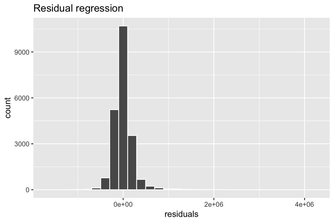
- What is the mean of the residuals? How do you interpret this?
kc_house %>%
  summarise(resid_mean = mean(residuals))
# A tibble: 1 x 1
resid_mean
<dbl>
1 -0.000000151- Now, create a new column called
residuals_abswhich shows the absolute value of the residuals (hint: use theabs()function).
kc_house <- kc_house %>%
mutate(residuals_abs = abs(price_glm$residuals))- Create a histogram of the absolute value of the residuals.
ggplot(data = kc_house,
       aes(x = residuals_abs)) +
  geom_histogram(col = "white") +
  labs(title = "Residual regression")
`stat_bin()` using `bins = 30`. Pick better value with `binwidth`.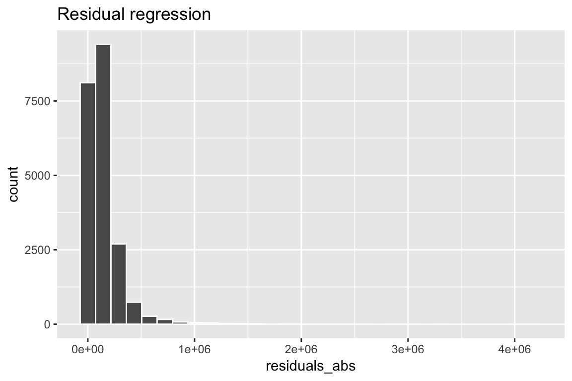
- What is the mean of the absolute value of the residuals? How do you interpret this? In general, do you think you can predict the price of a house very well based on the features in your regression model?
kc_house %>%
  summarise(resid_abs_mean = mean(residuals_abs))
# A tibble: 1 x 1
resid_abs_mean
<dbl>
1 144018.# On average, the model's fitted values are off by 144,018. So the model isn't terribly accurate on average.X - Challenges
- Which zipcode has the highest percentage of houses on the waterfront? (Hint: group by zipcode, calculate the percentage of houses on the waterfront using
mean(), then sort the data in descending order) witharrange(), then select the first row withslice(). Once you find it, try searching for that zipcode on Google Maps and see if its location makes sense!
kc_house %>%
  group_by(zipcode) %>%
  summarise(waterfront_p = mean(waterfront)) %>%
  arrange(desc(waterfront_p)) %>%
  slice(1)
# A tibble: 1 x 2
zipcode waterfront_p
<dbl> <dbl>
1 98070 0.203- Which house had the highest price to living space ratio? To answer this, create a new variable called
price_to_livingthat takesprice / living_sqm. Then, sort the data in descending order of this variable, and select the first row withslice()! What id value do you get?
kc_house %>%
  mutate(price_to_living = price / living_sqm) %>%
  arrange(desc(price_to_living)) %>%
  slice(1)
# A tibble: 1 x 29
id date price bedrooms bathrooms living_sqft lot_sqft
<chr> <dttm> <dbl> <dbl> <dbl> <dbl> <dbl>
1 6021… 2015-04-07 00:00:00 874950 2 1 1080 4000
# … with 22 more variables: floors <dbl>, waterfront <dbl>, view <dbl>,
# condition <dbl>, grade <dbl>, above_sqft <dbl>, basement_sqft <dbl>,
# built_yr <dbl>, renovated_yr <dbl>, zipcode <dbl>, lat <dbl>,
# long <dbl>, sqft_living15 <dbl>, sqft_lot15 <dbl>, living_sqm <dbl>,
# above_sqm <dbl>, basement_sqm <dbl>, total_sqm <dbl>, mansion <chr>,
# residuals <dbl>, residuals_abs <dbl>, price_to_living <dbl>- Which are the top 10 zip codes in terms of mean housing prices? To answer this, group the data by zipcode, calculate the mean price, arrange the dataset in descending order of mean price, then select the top 10 rows!
kc_house %>%
  group_by(zipcode) %>%
  summarise(price_mean = mean(price)) %>%
  arrange(desc(price_mean)) %>%
  slice(1:10)
# A tibble: 10 x 2
zipcode price_mean
<dbl> <dbl>
1 98039 2160607.
2 98004 1355927.
3 98040 1194230.
4 98112 1095499.
5 98102 901258.
6 98109 879624.
7 98105 862825.
8 98006 859685.
9 98119 849448.
10 98005 810165.- Create the following dataframe exactly as it appears.
| built_yr | N | price_mean | price_max | living_sqm_mean |
|---|---|---|---|---|
| 1990 | 320 | 563966 | 3640900 | 234 |
| 1991 | 224 | 630441 | 5300000 | 244 |
| 1992 | 198 | 548169 | 2480000 | 223 |
| 1993 | 202 | 556612 | 3120000 | 226 |
| 1994 | 249 | 486834 | 2880500 | 209 |
| 1995 | 169 | 577771 | 3200000 | 224 |
| 1996 | 195 | 639534 | 3100000 | 240 |
| 1997 | 177 | 606058 | 3800000 | 234 |
| 1998 | 239 | 594159 | 1960000 | 241 |
kc_house %>%
  filter(built_yr >= 1990 & built_yr < 1999) %>%
  group_by(built_yr) %>%
  summarise(N = n(),
            price_mean = mean(price),
            price_max = max(price),
            living_sqm_mean = mean(living_sqm)) %>%
knitr::kable(digits = 0)| built_yr | N | price_mean | price_max | living_sqm_mean |
|---|---|---|---|---|
| 1990 | 320 | 563966 | 3640900 | 234 |
| 1991 | 224 | 630441 | 5300000 | 244 |
| 1992 | 198 | 548169 | 2480000 | 223 |
| 1993 | 202 | 556612 | 3120000 | 226 |
| 1994 | 249 | 486834 | 2880500 | 209 |
| 1995 | 169 | 577771 | 3200000 | 224 |
| 1996 | 195 | 639534 | 3100000 | 240 |
| 1997 | 177 | 606058 | 3800000 | 234 |
| 1998 | 239 | 594159 | 1960000 | 241 |
- Create a regression object called
living_glmpredicting the amount of living space (living_sqm) as a function ofbedrooms,bathrooms,waterfront, andbuilt_yr. Explore the object withnames()andsummary(). Which variables seem to predict living space?
living_glm <- glm(formula = living_sqm ~ bedrooms + bathrooms + waterfront + built_yr,
                  data = kc_house)

names(living_glm)
[1] "coefficients" "residuals" "fitted.values"
[4] "effects" "R" "rank"
[7] "qr" "family" "linear.predictors"
[10] "deviance" "aic" "null.deviance"
[13] "iter" "weights" "prior.weights"
[16] "df.residual" "df.null" "y"
[19] "converged" "boundary" "model"
[22] "call" "formula" "terms"
[25] "data" "offset" "control"
[28] "method" "contrasts" "xlevels" summary(living_glm)
Call:
glm(formula = living_sqm ~ bedrooms + bathrooms + waterfront +
    built_yr, data = kc_house)

Deviance Residuals:
   Min      1Q  Median      3Q     Max
-705.7   -32.0    -4.9    25.7   566.1

Coefficients:
            Estimate Std. Error t value Pr(>|t|)
(Intercept) 219.6403    27.7140    7.93  2.4e-15 ***
bedrooms     23.1621     0.4532   51.11  < 2e-16 ***
bathrooms    71.3214     0.6294  113.31  < 2e-16 ***
waterfront   62.5121     4.1476   15.07  < 2e-16 ***
built_yr     -0.1297     0.0143   -9.09  < 2e-16 ***
---
Signif. codes:  0 '***' 0.001 '**' 0.01 '*' 0.05 '.' 0.1 ' ' 1

(Dispersion parameter for gaussian family taken to be 2750)

    Null deviance: 157675161  on 21612  degrees of freedom
Residual deviance:  59420739  on 21608  degrees of freedom
AIC: 232503

Number of Fisher Scoring iterations: 2- The
chisq.test()function allows you to do conduct a chi square test testing the relationship between two nominal variables. Look at the help menu to see how the function works. Then, conduct a chi-square test to see if there is a relationship between whether a house is on the waterfront and the grade of the house. Do houses on the waterfront tend to have higher (or lower) grades than houses not on the waterfront?
# First look at a table

table(kc_house$waterfront, kc_house$grade)
       1    3    4    5    6    7    8    9   10   11   12   13
  0    1    3   29  238 2026 8958 6028 2590 1106  379   79   13
  1    0    0    0    4   12   23   40   25   28   20   11    0
chisq.test(table(kc_house$waterfront, kc_house$grade))
    Pearson's Chi-squared test

data:  table(kc_house$waterfront, kc_house$grade)
X-squared = 300, df = 10, p-value <2e-16
Examples
# Analysing with dplyr and tidyr ---------------------------

library(tidyverse)    # Load tidyverse for dplyr
library(broom)        # For tidy results
library(rsq)          # For r-squared values

# Load baselers data
baselers <- read_csv("1_Data/baselers.txt")

# No grouping variables

bas <- baselers %>%
  summarise(
    age_mean = mean(age, na.rm = TRUE),
    income_median = median(income, na.rm = TRUE),
    N = n()
  )

# One grouping variable
bas_sex <- baselers %>%
  group_by(sex) %>%
  summarise(
    age_mean = mean(age, na.rm = TRUE),
    income_median = median(income, na.rm = TRUE),
    N = n()
  )

bas_sex

# Two grouping variables
bas_sex_ed <- baselers %>%
  group_by(sex, education) %>%
  summarise(
    age_mean = mean(age, na.rm = TRUE),
    income_median = median(income, na.rm = TRUE),
    N = n()
  )

# Advanced scoping

# Calculate mean of ALL numeric variables
baselers %>%
  group_by(sex, education) %>%
  summarise_if(is.numeric, mean, na.rm = TRUE)


# Examples of hypothesis tests on the diamonds -------------

# First few rows of the diamonds data

diamonds


# 2-sample t- test ---------------------------

# Q: Is there a difference in the carats of color = E and color = I diamonds?

htest_B <- t.test(formula = carat ~ color,     # DV ~ IV
                   alternative = "two.sided",  # Two-sided test
                   data = diamonds,         # The data
                   subset = color %in% c("E", "I")) # Compare Diet 1 and Diet 2

htest_B  # Print result

# Regression ----------------------------

# Q: Create regression equation predicting price by carat, depth, table, and x

price_glm <- glm(formula = price ~ carat + depth + table + x,
                  data = diamonds)

# Print coefficients
price_glm$coefficients

# Tidy version
tidy(price_glm)

# Extract R-Squared
rsq(price_glm)
Datasets
| File | Rows | Columns | Description |
|---|---|---|---|
| kc_house.csv | 21613 | 21 | House sale prices for King County between May 2014 and May 2015. |
First 5 rows and 5 columns of kc_house.csv
| id | date | price | bedrooms | bathrooms |
|---|---|---|---|---|
| 6762700020 | 2014-10-13 | 7700000 | 6 | 8.00 |
| 9808700762 | 2014-06-11 | 7062500 | 5 | 4.50 |
| 9208900037 | 2014-09-19 | 6885000 | 6 | 7.75 |
| 2470100110 | 2014-08-04 | 5570000 | 5 | 5.75 |
| 8907500070 | 2015-04-13 | 5350000 | 5 | 5.00 |
Functions
Packages
| Package | Installation | Description |
|---|---|---|
tidyverse |
install.packages("tidyverse") |
A collection of packages for data science, including dplyr, ggplot2 and others |
broom |
install.packages("broom") |
Provides ‘tidy’ outputs from statistical objects. |
rsq |
install.packages("rsq") |
Returns r-squared statistics from glm objects. |
Functions
Wrangling
| Function | Package | Description |
|---|---|---|
rename() |
dplyr |
Rename columns |
select() |
dplyr |
Select columns based on name or index |
filter() |
dplyr |
Select rows based on some logical criteria |
arrange() |
dplyr |
Sort rows |
mutate() |
dplyr |
Add new columns |
case_when() |
dplyr |
Recode values of a column |
group_by(), summarise() |
dplyr |
Group data and then calculate summary statistics |
left_join() |
dplyr |
Combine multiple data sets using a key column |
Statistical Tests
| Function | Package | Hypothesis Test |
|---|---|---|
glm(), lm() |
base |
Generalized linear model and linear model |
t.test() |
base |
One and two sample t-test |
wilcox.test() |
base |
Wilcoxon test |
cor.test() |
base |
Correlation test |
chisq.test |
base |
Chi-square tests for frequency tables |
Other
| Function | Package | Description |
|---|---|---|
tidy() |
broom |
Converts statistical objects to ‘tidy’ dataframes of key results |
rsq() |
rsq |
Returns r-squared statistics from glm objects |
Resources
dplyr vignette
See the full dplyr vignette with lots of wrangling tips and tricks.
Cheatsheets
from R Studio