Case study: Financial
R for Data Science
Basel R Bootcamp

Basel R Bootcamp

adapted from static.memrise.com
Overview
In this case study, you will analyse historic data of three major stock indices, the Dow Jones, the DAX, and the Nikkei, in relation to the exchange rates between the US dollar, the Euro, and the Yen. Using this data, you will address several questions.
- How large was the impact of the recent financial crisis on the respective stock markets?
- How correlated is the development between the stock markets?
- What is the relationship between stock market returns and exchange rates?
To address these questions, you will import several data files, using various function parameters to match the idiosyncrasies of the data. You will merge the data files into a single data frame, and mutate the data to reflect changes in index price and exchange rate. You will analyze correlations of stock indices among themselves and to exchange rates and create illustrative plots for each of the analyses.
Below you will find several tasks that will guide you through these steps. For the most part these tasks require you to make use of what you have learned in the sessions Data, Wrangling, Analysing, and Plotting.
Tasks
A - Getting setup
Open your
BaselRBootcampR project. It should already have the folders1_Dataand2_Code. Inside of the1_Datafolder, you should have all of the data sets listed in the Datasets section above!Open a new R script and save it as a new file in your
Rfolder calledfinancial_casestudy.R. At the top of the script, using comments, write your name and the date. Then, load thetidyversepackage. Here’s how the top of your script should look:
## My Name
## The Date
## Financial Data - Case Study

library(tidyverse)
B - Data
In this practical, you will load three external data sets
\^DJI.csv,\^GDAXI.csv, and\^N225.csv. Unfortunately, two of these data files are not yet tidy. Specifically,\^GDAXI.csvand\^N225.csvinclude a specific character string to represent missings in the data and is not identify by R as such. To identify theNA-character string in the data open one of them in a text viewer, (via RStudio or a word processor such as textedit). Do you see the string value that indicates missing data?Once you have identified the character string for missing data, us the
read_csv()function to load in the stock index data sets, “^DJI.csv”, “^GDAXI.csv”, and “^N225.csv”, from your1_Datafolder. In so doing, set an explicitna-argument to account for the fact that “^GDAXI.csv” “^N225.csv” use a specific character string to represent missings in the data.
# Load index data from local data folder
dow <- read_csv(file = '1_Data/^DJI.csv')
Parsed with column specification:
cols(
Date = col_date(format = ""),
Open = col_double(),
High = col_double(),
Low = col_double(),
Close = col_double(),
`Adj Close` = col_double(),
Volume = col_double()
)dax <- read_csv(file = '1_Data/^GDAXI.csv', na = 'null')Parsed with column specification:
cols(
Date = col_date(format = ""),
Open = col_double(),
High = col_double(),
Low = col_double(),
Close = col_double(),
`Adj Close` = col_double(),
Volume = col_double()
)nik <- read_csv(file = '1_Data/^N225.csv', na = 'null')Parsed with column specification:
cols(
Date = col_date(format = ""),
Open = col_double(),
High = col_double(),
Low = col_double(),
Close = col_double(),
`Adj Close` = col_double(),
Volume = col_double()
)Look at each dataset using the
View()function, were the data loaded correctly and are the missing values represented appropriately?Load in the exchange rate data sets,
euro-dollar.txtandyen-dollar.txt, from the1_Datafolder as two new objects calledeur_usdandyen_usd. To do this, use theread_delim()-function and\tas thedelim-argument, telling R that the data is tab-delimited.
# Load data
eur_usd <- read_delim(file = 'XX/XX',
                      delim = 'XX')

yen_usd <- read_delim(file = 'XX/XX',
                      delim = 'XX')
# Load exchange rate data from local data folder
eur_usd <- read_delim(file = '1_Data/euro-dollar.txt', delim = '\t')Parsed with column specification:
cols(
`04 Jan 1999` = col_character(),
`1.186669` = col_double()
)yen_usd <- read_delim(file = '1_Data/yen-dollar.txt', delim = '\t')Parsed with column specification:
cols(
`02 Jan 1990` = col_character(),
`0.006838` = col_double()
)- Print the
eur_usdandyen_usdobjects. Are all the data types and variable names correct? Not quite, right?
# print exchange rate data sets
eur_usd
# A tibble: 6,545 x 2
`04 Jan 1999` `1.186669`
<chr> <dbl>
1 05 Jan 1999 1.18
2 06 Jan 1999 1.16
3 07 Jan 1999 1.17
4 08 Jan 1999 1.16
5 11 Jan 1999 1.15
6 12 Jan 1999 1.16
7 13 Jan 1999 1.17
8 14 Jan 1999 1.17
9 15 Jan 1999 1.16
10 18 Jan 1999 1.16
# … with 6,535 more rowsyen_usd# A tibble: 8,764 x 2
`02 Jan 1990` `0.006838`
<chr> <dbl>
1 03 Jan 1990 0.00686
2 04 Jan 1990 0.00698
3 05 Jan 1990 0.00695
4 08 Jan 1990 0.00694
5 09 Jan 1990 0.00689
6 10 Jan 1990 0.00688
7 11 Jan 1990 0.00688
8 12 Jan 1990 0.00688
9 16 Jan 1990 0.00687
10 17 Jan 1990 0.00687
# … with 8,754 more rows- To fix the data sp that they have appropriate variable names, load the data again and use the
col_names-argument to explicitly assign the column names to beDateandRate. This will prevent R to take names from the first row of the data.
# Load data again, but specifying the column names explicitly
eur_usd <- read_delim(file = 'XX/XX',
                      delim = 'XX',
                      col_names = c('XX', 'XXX'))

yen_usd <- read_delim(file = 'XX/XX',
                      delim = 'XX',
                      col_names = c('XX', 'XX'))
# load data specifying col_names
eur_usd <- read_delim(file = '1_Data/euro-dollar.txt',
delim = '\t',
col_names = c('Date', 'Rate'))Parsed with column specification:
cols(
Date = col_character(),
Rate = col_double()
)yen_usd <- read_delim(file = '1_Data/yen-dollar.txt',
delim = '\t',
col_names = c('Date', 'Rate'))Parsed with column specification:
cols(
Date = col_character(),
Rate = col_double()
)Print your
eur_usdandyen_usdobjects. Do they look ok? Do you now see the column names you specified?Look closely at the print out of your objects: what class is your
Datecolumn represented as?
# change Date to date type in both datasets
eur_usd <- eur_usd %>%
  mutate(Date = parse_date(Date, format = '%d %b %Y'))

yen_usd <- yen_usd %>%
mutate(Date = parse_date(Date, format = '%d %b %Y'))- Print your
eur_usdandyen_usdobjects again, how do they look? Do they have the correct names and column classes?
C - Wrangling
- Before we can begin the analysis of the data, we to join the individual data frames into a single data frame called
financial_datathat contains only the dates variable (Date), the stock index (unadjusted) closing prices (Close), as well as the exchange rates. Begin by joiningdowanddaxusinginner_join(), selecting only theDateandClosevariables of each data frame. See the code below to help you do this.
# create single data frame
financial <- dow %>%
  select(Date,Close) %>%
  inner_join(dax %>% select(Date, Close), by = 'Date')
financial
# A tibble: 7,577 x 3
Date Close.x Close.y
<date> <dbl> <dbl>
1 1987-12-30 1950. 1005.
2 1987-12-31 1939. NA
3 1988-01-04 2015. 956.
4 1988-01-05 2032. 996.
5 1988-01-06 2038. 1006.
6 1988-01-07 2052. 1014.
7 1988-01-08 1911. 1027.
8 1988-01-11 1945. 988.
9 1988-01-12 1929. 987.
10 1988-01-13 1925. 966.
# … with 7,567 more rows- Inspect the data! What has R done with the names of the two
Closevariables? Run the code again, this time using thesuffix-argument to give both variables suffixes preserve the origin of these variables, e.g.,suffix = c(_dow','_dax').
# create single data frame
financial <- dow %>%
  select(Date,Close) %>%
  inner_join(dax %>% select(Date, Close),
            by = 'Date',
             suffix = c('_dow','_dax'))

# Print the result
financial
# A tibble: 7,577 x 3
Date Close_dow Close_dax
<date> <dbl> <dbl>
1 1987-12-30 1950. 1005.
2 1987-12-31 1939. NA
3 1988-01-04 2015. 956.
4 1988-01-05 2032. 996.
5 1988-01-06 2038. 1006.
6 1988-01-07 2052. 1014.
7 1988-01-08 1911. 1027.
8 1988-01-11 1945. 988.
9 1988-01-12 1929. 987.
10 1988-01-13 1925. 966.
# … with 7,567 more rows- Ok the data should look better now! Now that you know how to join two data sets, repeat the steps until all five data sets are included in
financial. Remember, we only want the dates variable (Date), the stock index (unadjusted) closing prices (Close). Note if you have trouble fixing all variables names using thesuffix-argument you can also take of this at the end usingrename().
financial <- financial %>%
  inner_join(nik %>% select(Date, Close), by = 'Date') %>%
  inner_join(eur_usd, by = 'Date') %>%
  inner_join(yen_usd, by = 'Date', suffix = c('_eur', '_yen')) %>%
rename(Close_nik = Close)- Alright, now let’s create
changevariables that show how the exchange rates and stock indices have moved. Use themutate- and thediff()-function. Thediffcomputes the differences between every adjacent pair of entries in a vector. As this results in one fewer differences than there values in the vector add anNAat the first position of the change variable à lac(NA, diff(my_variable)).
# create variables representing day-to-day changes
financial <- financial %>%
  mutate(
  Close_dow_change = c(NA, diff(Close_dow)),
  Close_dax_change = c(NA, diff(Close_dax)),
  Close_nik_change = c(NA, diff(Close_nik)),
  Rate_eur_change = c(NA, diff(Rate_eur)),
  Rate_yen_change = c(NA, diff(Rate_yen))
)- We will be mainly interested in how stock prices and exchange rates change over the course of a year. To create a variable that codes the year
mutate()andlubridate::year(Date), which will extract fromDatethe year information.
# load lubridate
library(lubridate)
Attaching package: 'lubridate'The following object is masked from 'package:base':
date# create year variable
financial <- financial %>%
mutate(year = year(Date))- Finally, we want the data in the “long”, instead of the current “wide” format. Call this dataset
financial_long. In long formats variables occupy different rows rather than columns. To this using thegather()-function. Hint: The first two arguments to thegather-function specify the names of the new variables, the third and fourth specify the names of the variables whose format you would like to change (minus in front is intentional). Check out the example in the?gather-help file.
# create long version of data frame
financial_long <- financial %>%
                gather(variable,
                       value,
                       -XXX,
                       -XXX)
# create long version of data frame
financial_long <- financial %>%
gather(variable,
value,
-Date,
-year)
financial_long# A tibble: 45,920 x 4
Date year variable value
<date> <dbl> <chr> <dbl>
1 1999-01-04 1999 Close_dow 9184.
2 1999-01-05 1999 Close_dow 9311.
3 1999-01-06 1999 Close_dow 9545.
4 1999-01-07 1999 Close_dow 9538.
5 1999-01-08 1999 Close_dow 9643.
6 1999-01-11 1999 Close_dow 9620.
7 1999-01-12 1999 Close_dow 9475.
8 1999-01-13 1999 Close_dow 9350.
9 1999-01-14 1999 Close_dow 9121.
10 1999-01-15 1999 Close_dow 9341.
# … with 45,910 more rows- Now your data is tidy proper (at least with regard to the analyses required here)! Go ahead an explore the data a bit by printing it and/or using
View()
D - Analysing and Plotting
- Plot the development of each of the stock indices over the available time periods. First, select rows corresponding to the stock index prices. Then use the
ggplot()-function to start a plot. Then, MapDatetoxandvaluetoyin theaes()-function. And, finally, add ageom_line(). Does the plot look right?
# create long version of data frame
financial_long %>%
  filter(variable %in% c("Close_dow", "Close_dax", "Close_nik")) %>%
ggplot(mapping = aes(x = Date, y = value)) +
  geom_line()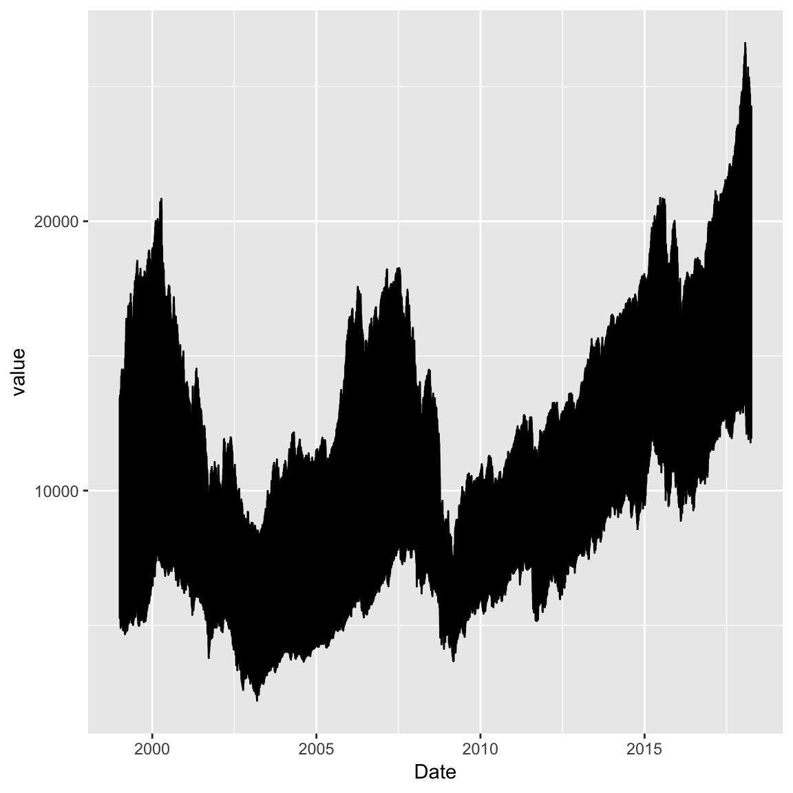
- It looks like the values of the three stock indices were somehow overlayering each other. Use
+ facet_grid(~variable)to show them in different plotting facets. Also give it a slightly nicer appearance using+ theme_light()What does the plot tell you? Has there been a particular drop in any year?
# create long version of data frame
financial_long %>%
  filter(variable %in% c("Close_dow", "Close_dax", "Close_nik")) %>%
ggplot(mapping = aes(x = Date, y = value)) +
  geom_line() +
  facet_grid(~variable) +
  theme_light()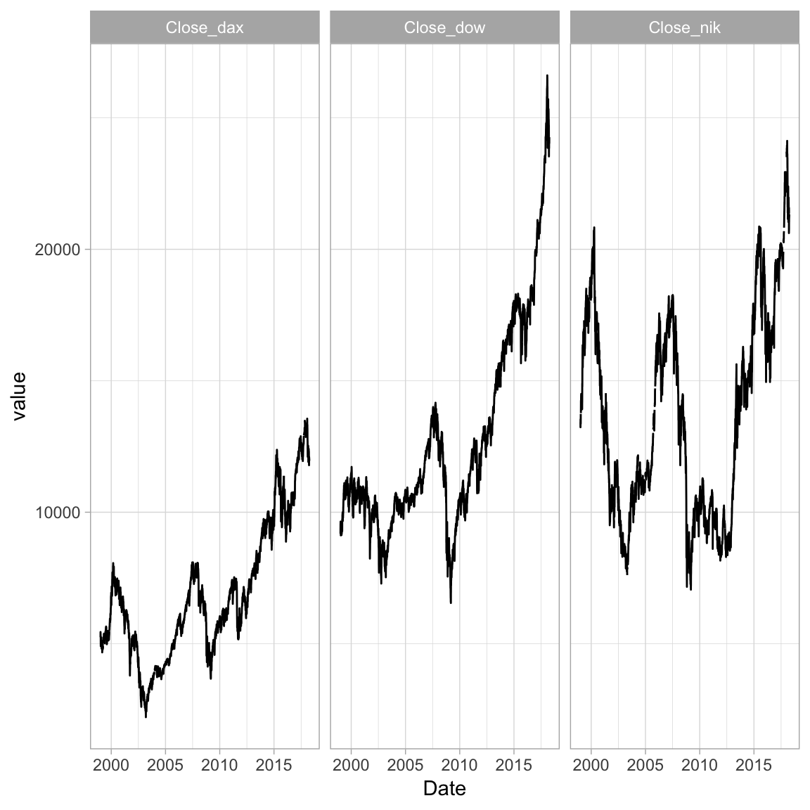
- Calculate the overall stock index price change per year. To do this, use
group_by()andsummarise()on the stock index change variables. Use the basicsum()-function insidesummarise()to compute the overall change in the year. In doing this, don’t forget there wereNA’s in two of the stock index price variables. Check out the result! When was the biggest drop in stock index prices?
# calculate aggregate change per year
aggregate_change <- financial %>%
  group_by(year) %>%
  summarize(
    mean_dow_change = sum(Close_dow_change),
    mean_dax_change = sum(Close_dax_change, na.rm = TRUE),
    mean_nik_change = sum(Close_nik_change, na.rm = TRUE)
)
aggregate_change
# A tibble: 20 x 4
year mean_dow_change mean_dax_change mean_nik_change
<dbl> <dbl> <dbl> <dbl>
1 1999 NA 1529. 5903.
2 2000 -709. -455. -5561.
3 2001 -766. -1254. -4436.
4 2002 -1680. -2112. -2235.
5 2003 2112. 718. 327.
6 2004 329. 180. 1335.
7 2005 -65.5 1108. 3219.
8 2006 1746. 1189. 1504.
9 2007 903. 1470. -1918.
10 2008 -4697. -3257. -6448.
11 2009 1880. 1147. 1513.
12 2010 1021. 957. -318.
13 2011 648. -1016. -1774.
14 2012 721. 1714. 1940.
15 2013 3566. 1940. 5896.
16 2014 1479. 253. 1159.
17 2015 -379. 937. 1583.
18 2016 2159. 738. 80.7
19 2017 4957. 1266. 3439.
20 2018 -455. -960. -2395. - The results up to now suggest that modern financial markets are closely intertwined, to the extent that a change in one market can bring about a change in the markets. Evaluate this aspect of financial markets by calculating all correlations between the three stock index change variables using the
cor()-function.cor()can take a data frame as an argument to produce the full correlation matrix among all variables in the data frame. This requires, however, that the data is stored in a “wide” format. Reactivate the old, widefinancialdata set and use it insidecor(). Before that select the variables you are interest in. Again, don’t forget about theNAs - there is an argument forcor()to deal with them. How closely are the stock indices related and which ones are most closely related?
financial %>%
  select(Close_dow_change, Close_dax_change, Close_nik_change) %>%
  cor(., use = 'complete.obs')
Close_dow_change Close_dax_change Close_nik_change
Close_dow_change 1.000 0.570 0.169
Close_dax_change 0.570 1.000 0.318
Close_nik_change 0.169 0.318 1.000- Evaluate the stability of the relationships between financial markets by calculating pair-wise correlations for each year using
group_byandsummarise(). Note that here you have to specify each pairwise correlation separately insidesummarise().
financial %>%
  group_by(year) %>%
  summarize(
    cor_dow_dax = cor(Close_dow_change, Close_dax_change, use = 'complete.obs'),
    cor_dow_nik = cor(Close_dow_change, Close_nik_change, use = 'complete.obs'),
    cor_dax_nik = cor(Close_dax_change, Close_nik_change, use = 'complete.obs')
)
# A tibble: 20 x 4
year cor_dow_dax cor_dow_nik cor_dax_nik
<dbl> <dbl> <dbl> <dbl>
1 1999 0.453 0.0730 0.192
2 2000 0.308 -0.0519 0.195
3 2001 0.667 0.255 0.287
4 2002 0.654 0.196 0.236
5 2003 0.695 0.127 0.249
6 2004 0.468 0.166 0.344
7 2005 0.390 0.0625 0.327
8 2006 0.594 0.100 0.266
9 2007 0.537 0.0874 0.394
10 2008 0.613 0.212 0.527
11 2009 0.732 0.175 0.260
12 2010 0.695 0.255 0.329
13 2011 0.796 0.185 0.351
14 2012 0.725 0.212 0.325
15 2013 0.566 0.161 0.256
16 2014 0.567 0.149 0.176
17 2015 0.538 0.254 0.295
18 2016 0.605 0.214 0.387
19 2017 0.554 0.367 0.395
20 2018 0.378 0.108 0.481- Another important aspect of financial markets are exchange rates between currencies. Generally, it is assumed that a strong economy translates into both a strong stock index and a strong currency relative to other currencies. For the end of this practical, let’s find out if that holds true our data. First, evaluate whether changes in exchange rates changes correlate with each other in the same way that stock indices did using the
cor-function.
financial %>%
  select(Rate_eur_change, Rate_yen_change) %>%
  cor(., use = 'complete.obs')
Rate_eur_change Rate_yen_change
Rate_eur_change 1.000 0.391
Rate_yen_change 0.391 1.000- Now, evaluate whether exchange rates vary as a function of the difference between stock indices. That is, for instance, does a large difference between Dow Jones and DAX translate into a strong Dollar relative to the EURO? According to the above intuition this should be the case. However, there is an alternative economic hypothesis. That is, foreign investors who benefit from a rise in stock index price may be motivated to sell their holdings and exchange them for their own currency to maintain a neutral position. This would, in effect, depreciate the currency at the same time as the stock index is outperforming, thus producing a negative relationship. What do you think? Ask the data.
financial %>%
  summarize(
    cor_dow_dax = cor(Close_dow - Close_dax, Rate_eur, use = 'complete.obs'),
    cor_dow_nik = cor(Close_dow - Close_nik, Rate_yen, use = 'complete.obs')
  )
# A tibble: 1 x 2
cor_dow_dax cor_dow_nik
<dbl> <dbl>
1 0.0869 0.569- Finally, evaluate the stability of the above relationship for each year separately. Can you make out a stable pattern? No? I guess it depends. As always.
financial %>%
  group_by(year) %>%
  summarize(
    cor_dow_dax = cor(Close_dow - Close_dax, Rate_eur, use = 'complete.obs'),
    cor_dow_nik = cor(Close_dow - Close_nik, Rate_yen, use = 'complete.obs')
  )
# A tibble: 20 x 3
year cor_dow_dax cor_dow_nik
<dbl> <dbl> <dbl>
1 1999 -0.639 -0.501
2 2000 -0.222 -0.479
3 2001 -0.393 -0.221
4 2002 0.162 -0.287
5 2003 0.772 -0.320
6 2004 0.253 0.427
7 2005 0.831 0.862
8 2006 0.776 0.0745
9 2007 -0.136 0.824
10 2008 0.825 0.788
11 2009 0.837 0.740
12 2010 0.714 0.932
13 2011 -0.334 0.459
14 2012 -0.248 0.727
15 2013 -0.235 0.898
16 2014 -0.856 0.781
17 2015 0.601 0.819
18 2016 -0.108 0.831
19 2017 0.784 0.629
20 2018 0.470 0.792 Datasets
| File | Rows | Columns | Description |
|---|---|---|---|
| ^DJI.csv | 8364 | 7 | Dow Jones Industrial stock history |
| ^GDAXI.csv | 7811 | 7 | DAX stock history |
| ^N225.csv | 13722 | 7 | Nikkei stock history |
| euro-dollar.txt | 6545 | 1 | Euro to dollar exchange rates |
| yen-dollar.txt | 8754 | 7 | Yen to dollar exchange rates |
Variables of data sets ^DJI.csv, ^GDAXI.csv, ^N225.csv
| Variable | Description |
|---|---|
| Date | Current day |
| Open | Day’s price when the stock exchange opened |
| High | Day’s highest price |
| Low | Day’s lowest price |
| Close | Day’s closing price |
| Adj Close | Adjusted closing price that has been amended to include any distributions and corporate actions that occurred at any time prior to the next day’s open |
Variables of data sets “euro-dollar.txt”, “yen-dollar.txt”
| Variable | Description |
|---|---|
| Date (currently unnamed) | Current day |
| Rate (currently unnamed) | Day’s exchange rate in terms of 1 US Dollar. E.g., a value of .75 means that the respective currency is worth a fraction of .75 of 1 US Dollar |
Functions
Packages
| Package | Installation |
|---|---|
tidyverse |
install.packages("tidyverse") |
haven |
install.packages("haven") |
Resources
Here are some articles relevant to the current case-study: